See any bugs/typos/confusing explanations? Open a GitHub issue. You can also comment below
★ See also the PDF version of this chapter (better formatting/references) ★
Multiparty secure computation II: Construction using Fully Homomorphic Encryption
In the last lecture we saw the definition of secure multiparty computation, as well as the compiler reducing the task of achieving security in the general (malicious) setting to the passive (honest-but-curious) setting. In this lecture we will see how using fully homomorphic encryption we can achieve security in the honest-but-curious setting.1 We focus on the two party case, and so prove the following theorem:
Assuming the LWE conjecture, for every two party functionality \(F\) there is a protocol computing \(F\) in the honest but curious model.
Before proving the theorem it might be worthwhile to recall what is actually the definition of secure multiparty computation, when specialized for the \(k=2\) and honest but curious case. The definition significantly simplifies here since we don’t have to deal with the possibility of aborts.
Let \(F\) be (possibly probabilistic) map of \(\{0,1\}^n\times \{0,1\}^n\) to \(\{0,1\}^n\times\{0,1\}^n\). A secure protocol for \(F\) is a two party protocol such for every party \(t\in \{1,2\}\), there exists an efficient “ideal adversary” (i.e., efficient interactive algorithm) \(S\) such that for every pair of inputs \((x_1,x_2)\) the following two distributions are computationally indistinguishable:
The tuple \((y_1,y_2,v)\) obtained by running the protocol on inputs \(x_1,x_2\), and letting \(y_1,y_2\) be the outputs of the two parties and \(v\) be the view (all internal randomness, inputs, and messages received) of party \(t\).
The tuple \((y_1,y_2,v)\) that is computed by letting \((y_1,y_2)=F(x_1,x_2)\) and \(v=S(x_t,y_t)\).
That is, \(S\), which only gets the input \(x_t\) and output \(y_t\), can simulate all the information that an honest-but-curious adversary controlling party \(t\) will view.
Constructing 2 party honest but curious computation from fully homomorphic encryption
Let \(F\) be a two party functionality. Lets start with the case that \(F\) is deterministic and that only Alice receives an output. We’ll later show an easy reduction from the general case to this one. Here is a suggested protocol for Alice and Bob to run on inputs \(x,y\) respectively so that Alice will learn \(F(x,y)\) but nothing more about \(y\), and Bob will learn nothing about \(x\) that he didn’t know before.
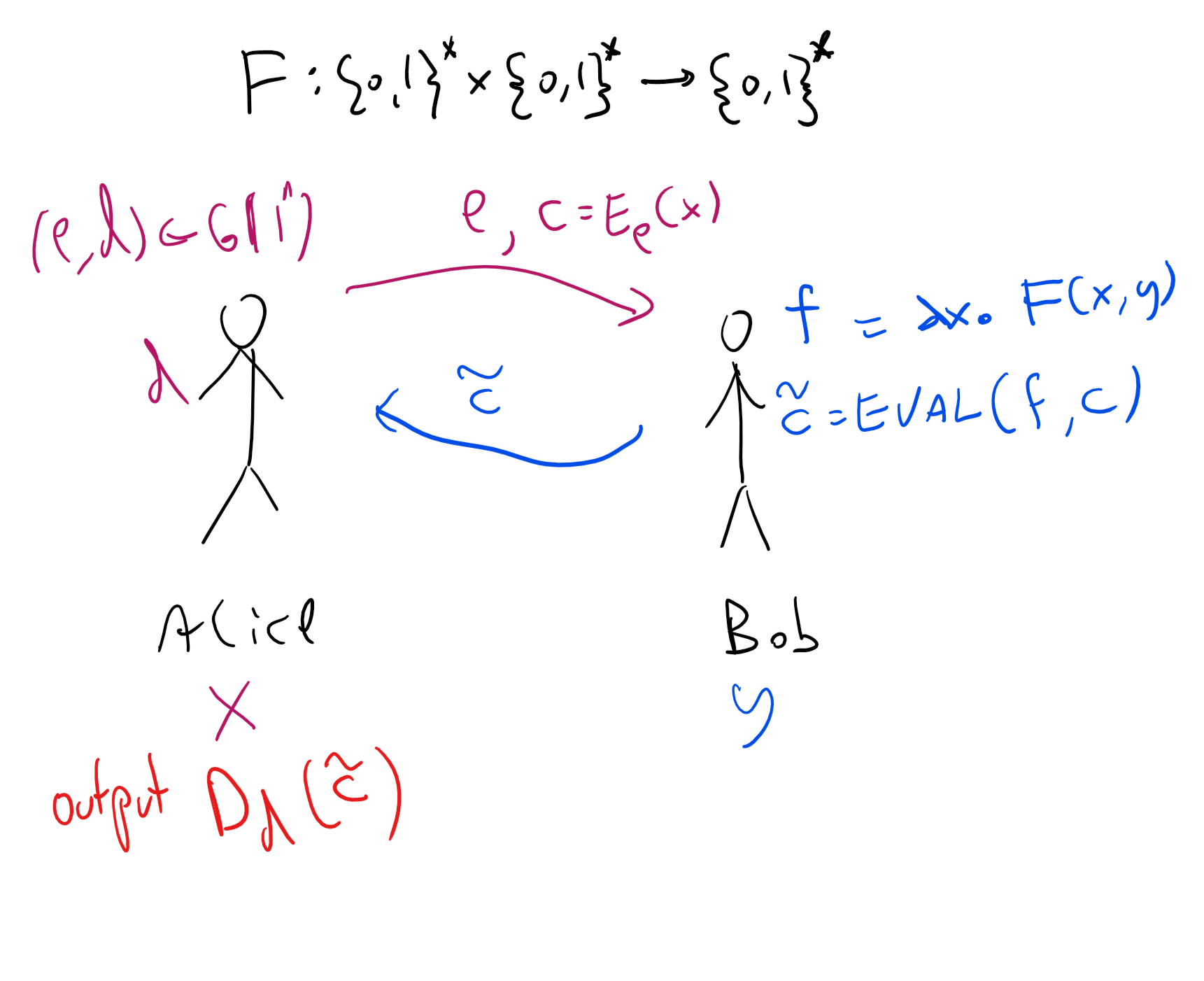
Protocol 2PC: (See Figure 17.1)
Assumptions: \((G,E,D,\ensuremath{\mathit{EVAL}})\) is a fully homomorphic encryption scheme.
Inputs: Alice’s input is \(x\in\{0,1\}^n\) and Bob’s input is \(y\in\{0,1\}^n\). The goal is for Alice to learn only \(F(x,y)\) and Bob to learn nothing.
Alice->Bob: Alice generates \((e,d)\leftarrow_R G(1^n)\) and sends \(e\) and \(c=E_e(x)\).
Bob->Alice: Bob defines \(f\) to be the function \(f(x)=F(x,y)\) and sends \(c'=\ensuremath{\mathit{EVAL}}(f,c)\) to Alice.
Alice’s output: Alice computes \(z=D_d(c')\).
First, note that if Alice and Bob both follow the protocol, then indeed at the end of the protocol Alice will compute \(F(x,y)\). We now claim that Bob does not learn anything about Alice’s input:
Claim B: For every \(x,y\), there exists a standalone algorithm \(S\) such that \(S(y)\) is indistinguishable from Bob’s view when interacting with Alice and their corresponding inputs are \((x,y)\).
Proof: Bob only receives a single message in this protocol of the form \((e,c)\) where \(e\) is a public key and \(c=E_e(x)\). The simulator \(S\) will generate \((e,d) \leftarrow_R G(1^n)\) and compute \((e,c)\) where \(c=E_e(0^n)\). (As usual \(0^n\) denotes the length \(n\) string consisting of all zeroes.) No matter what \(x\) is, the output of \(S\) is indistinguishable from the message Bob receives by the security of the encryption scheme. QED
(In fact, Claim B holds even against a malicious strategy of Bob- can you see why?)
We would now hope that we can prove the same regarding Alice’s security. That is prove the following:
Claim A: For every \(x,y\), there exists a standalone algorithm \(S\) such that \(S(y)\) is indistinguishable from Alice’s view when interacting with Bob and their corresponding inputs are \((x,y)\).
At this point, you might want to try to see if you can prove Claim A on your own. If you’re having difficulties proving it, try to think whether it’s even true.
So, it turns out that Claim A is not generically true. The reason is the following: the definition of fully homomorphic encryption only requires that \(\ensuremath{\mathit{EVAL}}(f,E(x))\) decrypts to \(f(x)\) but it does not require that it hides the contents of \(f\). For example, for every FHE, if we modify \(\ensuremath{\mathit{EVAL}}(f,c)\) to append to the ciphertext the first \(100\) bits of the description of \(f\) (and have the decryption algorithm ignore this extra information) then this would still be a secure FHE.2 Now we didn’t exactly specify how we describe the function \(f(x)\) defined as \(x \mapsto F(x,y)\) but there are clearly representations in which the first \(100\) bits of the description would reveal the first few bits of the hardwired constant \(y\), hence meaning that Alice will learn those bits from Bob’s message.
Thus we need to get a stronger property, known as circuit privacy. This is a property that’s useful in other contexts where we use FHE. Let us now define it:
::: {.definition title=“Perfect circuit privacy” #perfectcircprivatedef} Let \(\mathcal{E}=(G,E,D,\ensuremath{\mathit{EVAL}})\) be an FHE. We say that \(\mathcal{E}\) satisfies perfect circuit privacy if for every \((e,d)\) output by \(G(1^n)\) and every function \(f:\{0,1\}^\ell\rightarrow\{0,1\}\) of \(poly(n)\) description size, and every ciphertexts \(c_1,\ldots,c_\ell\) and \(x_1,\ldots,x_\ell \in \{0,1\}\) such that \(c_i\) is output by \(E_e(x_i)\), the distribution of \(\ensuremath{\mathit{EVAL}}_e(f,c_1,\ldots,c_\ell)\) is identical to the distribution of \(E_e(f(x))\). That is, for every \(z\in\{0,1\}^*\), the probability that \(\ensuremath{\mathit{EVAL}}_e(f,c_1,\ldots,c_\ell)=z\) is the same as the probability that \(E_e(f(x))=z\). We stress that these probabilities are taken only over the coins of the algorithms \(\ensuremath{\mathit{EVAL}}\) and \(E\).
Perfect circuit privacy is a strong property, that also automatically implies that \(D_d(\ensuremath{\mathit{EVAL}}(f,E_e(x_1),\ldots,E_e(x_\ell)))=f(x)\) (can you see why?). In particular, once you understand the definition, the following lemma is a fairly straightforward exercise.
If \((G,E,D,\ensuremath{\mathit{EVAL}})\) satisfies perfect circuit privacy then if \((e,d) = G(1^n)\) then for every two functions \(f,f':\{0,1\}^\ell\rightarrow\{0,1\}\) of \(poly(n)\) description size and every \(x\in\{0,1\}^\ell\) such that \(f(x)=f'(x)\), and every algorithm \(A\),
Please stop here and try to prove Lemma 17.3
The algorithm \(A\) above gets the secret key as input, but still cannot distinguish whether the \(\ensuremath{\mathit{EVAL}}\) algorithm used \(f\) or \(f'\). In fact, the expression on the lefthand side of Equation 17.1 is equal to zero when the scheme satisfies perfect circuit privacy.
However, for our applications bounding it by a negligible function is enough. Hence, we can use the relaxed notion of “imperfect” circuit privacy, defined as follows:
Let \(\mathcal{E}=(G,E,D,\ensuremath{\mathit{EVAL}})\) be an FHE. We say that \(\mathcal{E}\) satisfies statistical circuit privacy if for every \((e,d)\) output by \(G(1^n)\) and every function \(f:\{0,1\}^\ell\rightarrow\{0,1\}\) of \(poly(n)\) description size, and every ciphertexts \(c_1,\ldots,c_\ell\) and \(x_1,\ldots,x_\ell \in \{0,1\}\) such that \(c_i\) is output by \(E_e(x_i)\), the distribution of \(\ensuremath{\mathit{EVAL}}_e(f,c_1,\ldots,c_\ell)\) is equal up to \(negl(n)\) total variation distance to the distribution of \(E_e(f(x))\).
That is,
where once again, these probabilities are taken only over the coins of the algorithms \(\ensuremath{\mathit{EVAL}}\) and \(E\).
If you find Definition 17.4 hard to parse, the most important points you need to remember about it are the following:
Statistical circuit privacy is as good as perfect circuit privacy for all applications, and so you can imagine the latter notion when using it.
Statistical circuit privacy can easier to achieve in constructions.
(The third point, which goes without saying, is that you can always ask clarifying questions in class, Piazza, sections, or office hours…)
Intuitively, circuit privacy corresponds to what we need in the above protocol to protect Bob’s security and ensure that Alice doesn’t get any information about his input that she shouldn’t have from the output of \(\ensuremath{\mathit{EVAL}}\), but before working this out, let us see how we can construct fully homomorphic encryption schemes satisfying this property.
Achieving circuit privacy in a fully homomorphic encryption
We now discuss how we can modify our fully homomorphic encryption schemes to achieve the notion of circuit privacy. In the scheme we saw, the encryption of a bit \(b\), whether obtained through the encryption algorithm or \(\ensuremath{\mathit{EVAL}}\), always had the form of a matrix \(C\) over \(\Z_q\) (for \(q=2^{\sqrt{n}}\)) where \(Cv = bv + e\) for some vector \(e\) that is “small” (e.g., for every \(i\), \(|e_i| < n^{polylog(n)}\ll q=2^{\sqrt{n}}\)). However, the \(\ensuremath{\mathit{EVAL}}\) algorithm was deterministic and hence this vector \(e\) is a function of whatever function \(f\) we are evaluating and someone that knows the secret key \(v\) could recover \(e\) and then obtain from it some information about \(f\). We want to make \(\ensuremath{\mathit{EVAL}}\) probabilistic and lose that information, and we use the following approach
To kill a signal, drown it in lots of noise
That is, if we manage to add some additional random noise \(e'\) that has magnitude much larger than \(e\), then it would essentially “erase” any structure \(e\) had. More formally, we will use the following lemma:
Let \(a\in \Z_q\) and \(T\in\mathbb{N}\) be such that \(aT<q/2\). If we let \(X\) be the distribution obtained by taking \(x \pmod q\) for an integer \(x\) chosen at random in \([-T,+T]\) and let \(X'\) be the distribution obtained by taking \(a+x \pmod q\) for \(x\) chosen in the same way, then
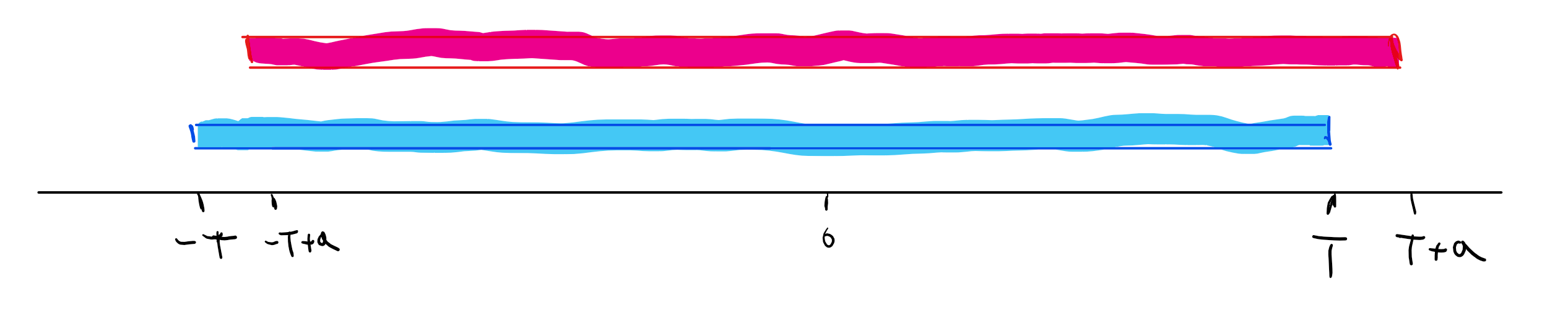
This has a simple “proof by picture”: consider the intervals \([-T,+T]\) and \([-T+a,+T+a]\) on the number line (see Figure 17.2). Note that the symmetric difference of these two intervals is only about a \(a/T\) fraction of their union. More formally, \(X\) is the uniform distribution over the \(2T+1\) numbers in the interval \([-T,+T]\) while \(X'\) is the uniform distribution over the shifted version of this interval \([-T+a,+T+a]\). There are exactly \(2|a|\) numbers which get probability zero under one of those distributions and probability \((2T+1)^{-1}<(2T)^{-1}\) under the other.
We will also use the following lemma:
If two distributions over numbers \(X\) and \(X'\) satisfy \(\Delta(X,X')=\sum_{y\in\Z}|\Pr[X=x]-\Pr[Y=y]|<\delta\) then the distributions \(X^m\) and \(X'^m\) over \(m\) dimensional vectors where every entry is sampled independently from \(X\) or \(X'\) respectively satisfy \(\Delta(X^m,X'^m) \leq m\delta\).
We omit the proof of Lemma 17.6 and leave it as an exercise to prove it using the hybrid argument. We will actually only use Lemma 17.6 for distributions above; you can obtain intuition for it by considering the \(m=2\) case where we compare the rectangles of the forms \([-T,+T]\times [-T,+T]\) and \([-T+a,+T+a]\times[-T+b,+T+b]\). You can see that their union has size roughly \(4T^2\) while their symmetric difference has size roughly \(2T\cdot 2a + 2T\cdot 2b\), and so if \(|a|,|b| \leq \delta T\) then the symmetric difference is roughly a \(2\delta\) fraction of the union.
We will not provide the full details, but together these lemmas show that \(\ensuremath{\mathit{EVAL}}\) can use bootstrapping to reduce the magnitude of the noise to roughly \(2^{n^{0.1}}\) and then add an additional random noise of roughly, say, \(2^{n^{0.2}}\) which would make it statistically indistinguishable from the actual encryption. Here are some hints on how to make this work: the idea is that in order to “re-randomize” a ciphertext \(C\) we need a very noisy encryption of zero and add it to \(C\). The normal encryption will use noise of magnitude \(2^{n^{0.2}}\) but we will provide an encryption of the secret key with smaller magnitude \(2^{n^{0.1}/polylog(n)}\) so we can use bootstrapping to reduce the noise. The main idea that allows to add noise is that at the end of the day, our scheme boils down to LWE instances that have the form \((c,\sigma)\) where \(c\) is a random vector in \(\Z_q^{n-1}\) and \(\sigma = \langle c,s \rangle+a\) where \(a \in [-\eta,+\eta]\) is a small noise addition. If we take any such input and add to \(\sigma\) some \(a' \in [-\eta',+\eta']\) then we create the effect of completely re-randomizing the noise. However, completely analyzing this requires non-trivial amount of care and work.
Bottom line: A two party secure computation protocol
Using the above we can obtain the following theorem:
If the LWE conjecture is true then there exists a tuple of polynomial-time randomized algorithms \((G,E,D,\ensuremath{\mathit{EVAL}},\ensuremath{\mathit{RERAND}})\) such that:
\((G,E,D,\ensuremath{\mathit{EVAL}})\) is a CPA secure fully-homomorphic encryption for one bit messages. That is, if \((d,e)=G(1^n)\) then for every Boolean circuit \(C\) with \(\ell\) inputs and one output, and \(x\in \{0,1\}^\ell\), the ciphertext \(c = \ensuremath{\mathit{EVAL}}_e(C, E_e(x_1),\ldots, E_e(x_\ell)\) has length \(n\) and \(D_d(c)=C(x)\) with probability one over the random choices of the algorithms \(E\) and \(\ensuremath{\mathit{EVAL}}\).
For every pair of keys \((e,d) =G(1^n)\) there are two distributions \(\mathcal{C}^0,\mathcal{C}^1\) over \(\{0,1\}^n\) such that:
For \(b\in \{0,1\}\), \(\Pr_{c \sim \mathcal{C}^b} [ D_d(c) = b ]=1\). That is, \(\mathcal{C}^b\) is distributed over ciphertexts that decrypt to \(b\).
For every ciphertext \(c \in \{0,1\}^n\) in the image of either \(E_e(\cdot)\) or \(\ensuremath{\mathit{EVAL}}_e(\cdot)\), if \(D_d(c)=b\) then \(\ensuremath{\mathit{RERAND}}_e(c)\) is statistically indistinguishable from \(\mathcal{C}^b\). That is, the output of \(\ensuremath{\mathit{RERAND}}_e(c)\) is a ciphertext that decrypts to the same plaintext as \(c\), but whose distribution is essentially independent of \(c\).
We do not include the full proof but the idea is we use our standard LWE-based FHE and to rerandomize a ciphertext \(c\) we will add to it an encryption of \(0\) (which will not change the corresponding plaintext) and an additional noise vector that would be of much larger magnitude than the original noise vector of \(c\), but still small enough so decryption succeeds.
Using the above re-randomizable encryption scheme, we can redefine \(\ensuremath{\mathit{EVAL}}\) to add a \(\ensuremath{\mathit{RERAND}}\) step at the end and achieve statistical circuit privacy. If we use Protocol 2PC with such a scheme then we get a two party computation protocol secure with respect to honest but curious adversaries. Using the compiler of Theorem 16.5 we obtain a proof of Theorem 16.3 for the two party setting:
If the LWE conjecture is true then for every (potentially randomized) functionality \(F:\{0,1\}^{n_1} \times \{0,1\}^{n_2} \rightarrow \{0,1\}^{m_1} \times \{0,1\}^{m_2}\) there exists a polynomial-time protocol for computing the functionality \(F\) secure with respect to potentially malicious adversaries.
Beyond two parties
We now sketch how to go beyond two parties. It turns out that the compiler of honest-but-curious to malicious security works just as well in the many party setting, and so the crux of the matter is to obtain an honest but curious secure protocol for \(k>2\) parties.
We start with the case of three parties - Alice, Bob, and Charlie. First, let us introduce some convenient notation (which is used in other settings as well).3 We will assume that each party initially generates private/public key pairs with respect to some fully homomorphic encryption (satisfying statistical circuit privacy) and sends them to the other parties. We will use \(\{ x \}_A\) to denote the encryption of \(x\in \{0,1\}^\ell\) using Alice’s public key (similarly \(\{ x \}_B\) and \(\{ x \}_C\) will denote the encryptions of \(x\) with respect to Bob’s and Charlie’s public key. We can also compose these and so denote by \(\{ \{ x \}_A \}_B\) the encryption under Bob’s key of the encryption under Alice’s key of \(x\).
With the notation above, Protocol 2PC can be described as follows:
Protocol 2PC: (Using BAN notation)
Inputs: Alice’s input is \(x\in\{0,1\}^n\) and Bob’s input is \(y\in\{0,1\}^n\). The goal is for Alice to learn only \(F(x,y)\) and Bob to learn nothing.
Alice->Bob: Alice sends \(\{ x \}_A\) to Bob. (We omit from this description the public key of Alice which can be thought of as being concatenated to the ciphertext).
Bob->Alice: Bob sends \(\{ f(x,y) \}_A\) to Alice by running \(\ensuremath{\mathit{EVAL}}_A\) on the ciphertext \(\{ x\}_A\) and the map \(x \mapsto F(x,y)\).
Alice’s output: Alice computes \(f(x,y)\)
We can now describe the protocol for three parties. We will focus on the case where the goal is for Alice to learn \(F(x,y,z)\) (where \(x,y,z\) are the private inputs of Alice, Bob, and Charlie, respectively) and for Bob and Charlie to learn nothing. As usual we can reduce the general case to this by running the protocol multiple times with parties switching the roles of Alice, Bob, and Charlie.
Protocol 3PC: (Using BAN notation)
Inputs: Alice’s input is \(x\in\{0,1\}^n\), Bob’s input is \(y\in\{0,1\}^n\), and Charlie’s input is \(z\in \{0,1\}^m\). The goal is for Alice to learn only \(F(x,y,z)\) and for Bob and Charlie to learn nothing.
Alice->Bob: Alice sends \(\{ x \}_A\) to Bob.
Bob–>Charlie: Bob sends \(\{ \{x\}_A , y \}_B\) to Charlie.
Charlie–>Bob: Charlie sends \(\{ \{ F(x,y,z) \}_A \}_B\) to Bob. Charlie can do this by running \(\ensuremath{\mathit{EVAL}}_B\) on the ciphertext and on the (efficiently computable) map \(c,y \mapsto \ensuremath{\mathit{EVAL}}_A(f_y,c)\) where \(f_y\) is the circuit \(x \mapsto F(x,y,z)\). (Please read this line several times!)
Bob–>Alice: Bob sends \(\{ F(x,y,z) \}_A\) to Alice by decrypting the ciphertext sent from Charlie.
Alice’s output: Alice computes \(F(x,y,z)\) by decrypting the ciphertext sent from Bob.
If the underlying encryption is a fully homomorphic statistically circuit private encryption then Protocol 3PC is a secure protocol for the functionality \((x,y,z) \mapsto (F(x,y,z),\bot,\bot)\) with respect to honest-but-curious adversaries.
Left to the reader :)
- ↩
This is by no means the only way to get multiparty secure computation. In fact, multiparty secure computation was known well before FHE was discovered. One common construction for achieving this uses a technique known as Yao’s Garbled Circuit.
- ↩
It’s true that strictly speaking, we allowed \(\ensuremath{\mathit{EVAL}}\)’s output to have length at most \(n\), while this would make the output be \(n+100\), but this is just a technicality that can be easily bypassed, for example by having a new scheme that on security parameter \(n\) runs the original scheme with parameter \(n/2\) (and hence will have a lot of “room” to pad the output of \(\ensuremath{\mathit{EVAL}}\) with extra bits).
- ↩
I believe this notation originates with Burrows–Abadi–Needham (BAN) logic though would be happy to get corrections/references.
Comments
Comments are posted on the GitHub repository using the utteranc.es app. A GitHub login is required to comment. If you don't want to authorize the app to post on your behalf, you can also comment directly on the GitHub issue for this page.
Compiled on 11/17/2021 22:36:20
Copyright 2021, Boaz Barak.

This work is
licensed under a Creative Commons
Attribution-NonCommercial-NoDerivatives 4.0 International License.
Produced using pandoc and panflute with templates derived from gitbook and bookdown.