Key derivation, protecting passwords, slow hashes, Merkle trees

Last lecture we saw the notion of cryptographic hash functions which are functions that behave like a random function, even in settings (unlike that of standard PRFs) where the adversary has access to the key that allows them to evaluate the hash function. Hash functions have found a variety of uses in cryptography, and in this lecture we survey some of their other applications. In some of these cases, we only need the relatively mild and well-defined property of collision resistance while in others we only know how to analyze security under the stronger (and not precisely well defined) random oracle heuristic.

Keys from passwords

We have seen great cryptographic tools, including PRFs, MACs, and CCA secure encryptions, that Alice and Bob can use when they share a cryptographic key of 128 bits or so. But unfortunately, many of the current users of cryptography are humans which, generally speaking, have extremely faulty memory capacity for storing large numbers. There are \(62^8 \approx 2^{48}\) ways to select a password of 8 upper and lower case letters + numbers, but some letter/numbers combinations end up being chosen much more frequently than others. Due to several large scale hacks, very large databases of passwords have been made public, and one estimate is that 91 percent of the passwords chosen by users are contained in a list of about \(1,000 \approx 2^{10}\) strings.

If we choose a password at random from some set \(D\) then the entropy of the password is simply \(\log_2 |D|\). However, estimating the entropy of real life passwords is rather difficult. For example, suppose that I use the winning Massachussets Mega-Lottery numbers as my password. A priori, my password consists of \(5\) numbers between \(1\) till \(75\) and so its entropy is \(\log_2 (75^5) \approx 31\). However, if an attacker knew that I did this, the entropy might be something like \(\log(520) \approx 9\) (since there were only 520 such numbers selected in the last 10 years). Moreover, if they knew exactly what draw I based my password on, then they would know it exactly and hence the entropy (from their point of view) would be zero. This is worthwhile to emphasize:

The entropy of a secret is always measured with respect to the attacker’s point of view.

The exact security of passwords is of course a matter of intense practical interest, but we will simply model the password as being chosen at random from some set \(D\subseteq\{0,1\}^n\) (which is sometimes called the “dictionary”). The set \(D\) is known to the attacker, but she has no information on the particular choice of the password.

Much of the challenge for using passwords securely relies on the distinction between offline and online attacks. If each guess for a password requires interacting online with a server, as is the case when typing a PIN number in the ATM, then even a weak password (such as a 4 digit PIN that at best provides \(13\) bits of entropy) can yield meaningful security guarantees, as typically an alarm would be raised after five or so failed attempts.
However, if the adversary has the ability to check offline whether a password is correct then the number of guesses they can try can be as high as the number of computing cycles at their disposal, which can easily run into the billions and so break passwords of \(30\) or more bits of entropy. (This is an issue we’ll return to after we learn about public key cryptography when we’ll talk about password authenticated key exchange.)

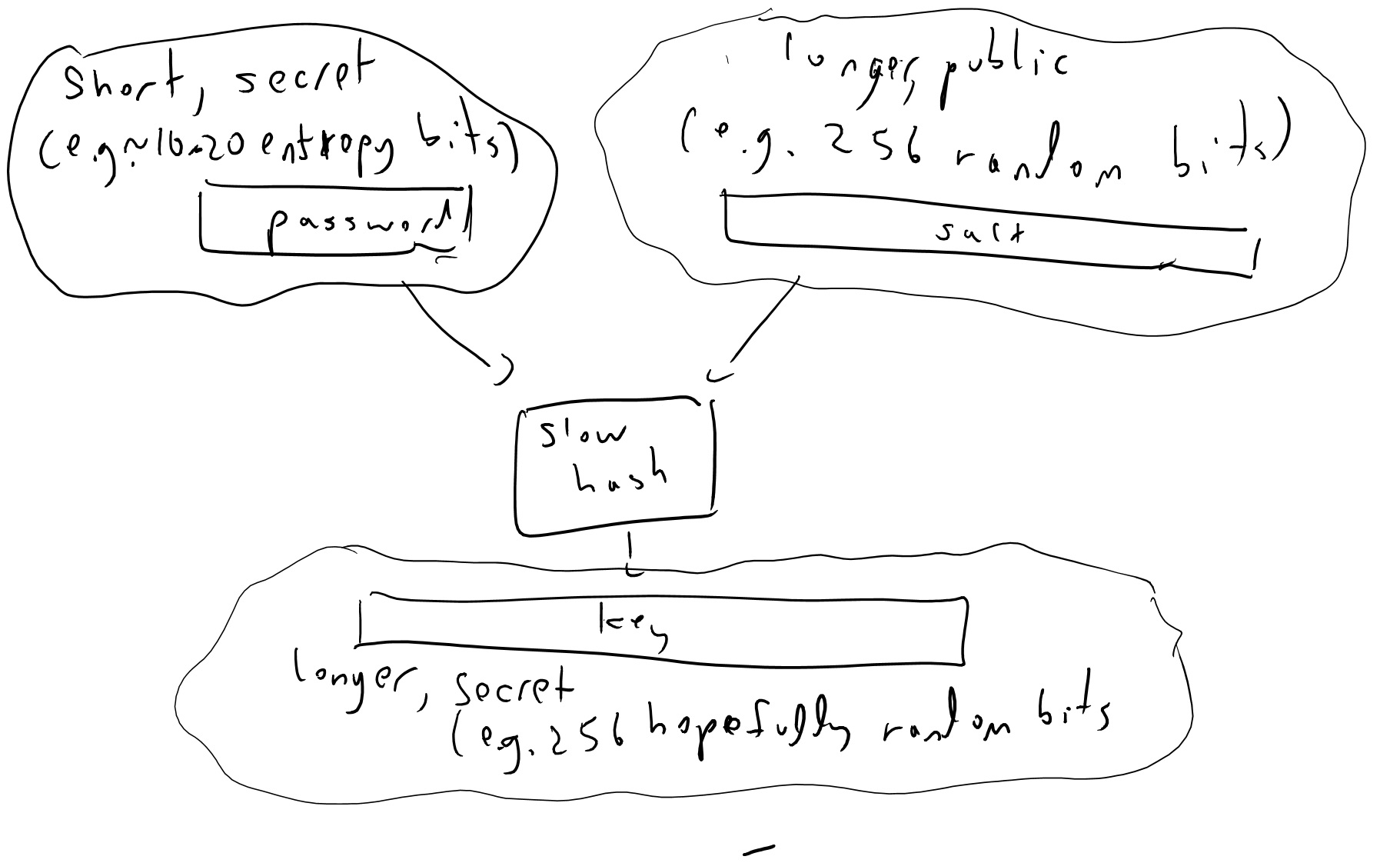
Consider a password manager application. In such an application, a user typically chooses a master password \(p_{master}\) which she can then use to access all her other passwords \(p_1,\ldots,p_t\). To enable her to do so without requiring online access to a server, the master password \(p_{master}\) is used to encrypt the other passwords. However to do that, we need to derive a key \(k_{master}\) from the password.

A classical approach is to simply use a cryptographic hash function \(H:\{0,1\}^*\rightarrow\{0,1\}^n\), and let \(k_{master} = H(p_{master})\). If we think of \(H\) as a random oracle and \(p_{master}\) as chosen randomly from \(D\), then as long as an attacker makes \(\ll |D|\) queries to the oracle, they are unlikely to make the query \(p_{master}\) and hence the value \(k_{master}\) will be completely random from their point of view.

However, since \(|D|\) is not too large, it might not be so hard to perform such \(|D|\) queries. For this reason, people typically use a deliberately slow hash function as a key derivation function. The rationale is that the honest user only needs to evaluate \(H\) once, and so could afford for it to take a while, while the adversary would need to evaluate it \(|D|\) times. For example, if \(|D|\) is about \(100,000\) and the honest user is willing to spend 1 cent of computation resources every time they need to derive \(k_{master}\) from \(p_{master}\), then we could set \(H(\cdot)\) so that it costs 1 cent to evaluate it and hence on average it will cost the adversary \(1,000\) dollars to recover it.

There are several approaches for trying to make \(H\) deliberately “slow” or “costly” to evaluate but the most popular and simplest one is to simply let \(H\) be obtained by iterating many times a basic hash function such as SHA-256. That is, \(H(x)=h(h(h(\cdots h(x))))\) where \(h\) is some standard (“fast”) cryptographic hash function and the number of iterations is tailored to be the largest one that the honest users can tolerate.¹

In fact, typically we will set \(k_{master} = H(p_{master}\| r)\) where \(r\) is a long random but public string known as a “salt” (see Figure 8.1). Including such a “salt” can be important to foiling an adversary’s attempts to amortize the computation costs, see the exercises.

Even when we don’t use one password to encrypt others, it is generally considered the best practice to never store a password in the clear but always in this “slow hashed and salted” form, so if the passwords file falls to the hands of an adversary it will be expensive to recover them.

Merkle trees and verifying storage.

Suppose that you outsource to the cloud storing your huge data file \(x\in\{0,1\}^N\). You now need the \(i^{th}\) bit of that file and ask the cloud for \(x_i\). How can you tell that you actually received the correct bit?

Ralph Merkle came up in 1979 with a clever solution, which is known as “Merkle hash trees”. The idea is the following (see Theorem 8.1): suppose we have a collision-resistant hash function \(h:\{0,1\}^{2n}\rightarrow\{0,1\}^n\), and think of the string \(x\) as composed of \(t\) blocks of size \(n\). We then hash every pair of consecutive blocks to transform \(x\) into a string \(x_1\) of \(t/2\) blocks, and continue in this way for \(\log t\) steps until we get a single block \(y\in\{0,1\}^n\). (Assume here \(t\) is a power of two for simplicity, though it doesn’t make much difference.)

Alice, who sends \(x\) to the cloud Bob, will keep the short block \(y\). Whenever Alice queries the value \(i\) she will ask for a certificate that \(x_i\) is indeed the right value. This certificate will consists of the block that contains \(i\), as well as all of the \(2\log t\) blocks that were used in the hash from this block to the root. The security of this scheme follows from the following simple theorem:

Proofs of Retrievability

The above provides a way to ensure Alice that the value retrieved from a cloud storage is correct, but how can Alice be sure that the cloud server still stores the values that she did not ask about?

A priori, you might think that she obviously can’t. If Bob is lazy, or short on storage, he could decide to store only some small fraction of \(x\) that he thinks Alice is more likely to query for. As long as Bob wasn’t unlucky and Alice doesn’t ask these queries, then it seems Bob could get away with this. In a proof of retrievability, first proposed by Juels and Kalisky in 2007, Alice would be able to get convinced that Bob does in fact store her data.

First, note that Alice can guarantee that Bob stores at least 99 percent of her data, by periodically asking him to provide answers (with proofs!) of the value of \(x\) at 100 or so random locations. The idea is that if Bob dropped more than 1 percent of the bits, then he’d be very likely to be caught “red handed” and get a question from Alice about a location he did not retain.

Now, if we used some redundancy to store \(x\) such as the RAID format, where it is composed of some small number \(c\) parts and we can recover any bit of the original data as long as at most one of the parts were lost, then we might hope that even if 1% of \(x\) was in fact lost by Bob, we could still recover the whole string. This is not a fool-proof guarantee since it could possibly be that the data lost by Bob was not confined to a single part. To handle this case one needs to consider generalizations of RAID known as “local reconstruction codes” or “locally decodable codes”. The paper by Dodis, Vadhan and Wichs is a good source for this; see also these slides by Seny Kamara for a more recent overview of the theory and implementations.

Entropy extraction

As we’ve seen time and again, randomness is crucial to cryptography. But how do we get these random bits we need? If we only have a small number \(n\) of random bits (e.g., \(n=128\) or so) then we can expand them to as large a number as we want using a pseudorandom generator, but where do we get those initial \(n\) bits from?

The approach used in practice is known as “harvesting entropy”. The idea is that we make great many measurements \(x_1,\ldots,x_m\) of events that are considered “unpredictable” to some extent, including mouse movements, hard-disk and network latency, sources of noise etc… and accumulate them in an entropy “pool” which would simply be some memory array. When we estimate that we have accumulated more than \(128\) bits of randomness, then we hash this array into a \(128\) bit string which we’ll use as a seed for a pseudorandom generator (see Figure 8.3).² Because entropy needs to be measured from the point of view of the attacker, this “entropy estimation” routine is a bit of a “black art” and there isn’t a very principled way to perform it. In practice people try to be very conservative (e.g., assume that there is only one bit of entropy for 64 bits of measurements or so) and hope for the best, which often works but sometimes also spectacularly fails, especially in embedded systems that do not have access to many of these sources.

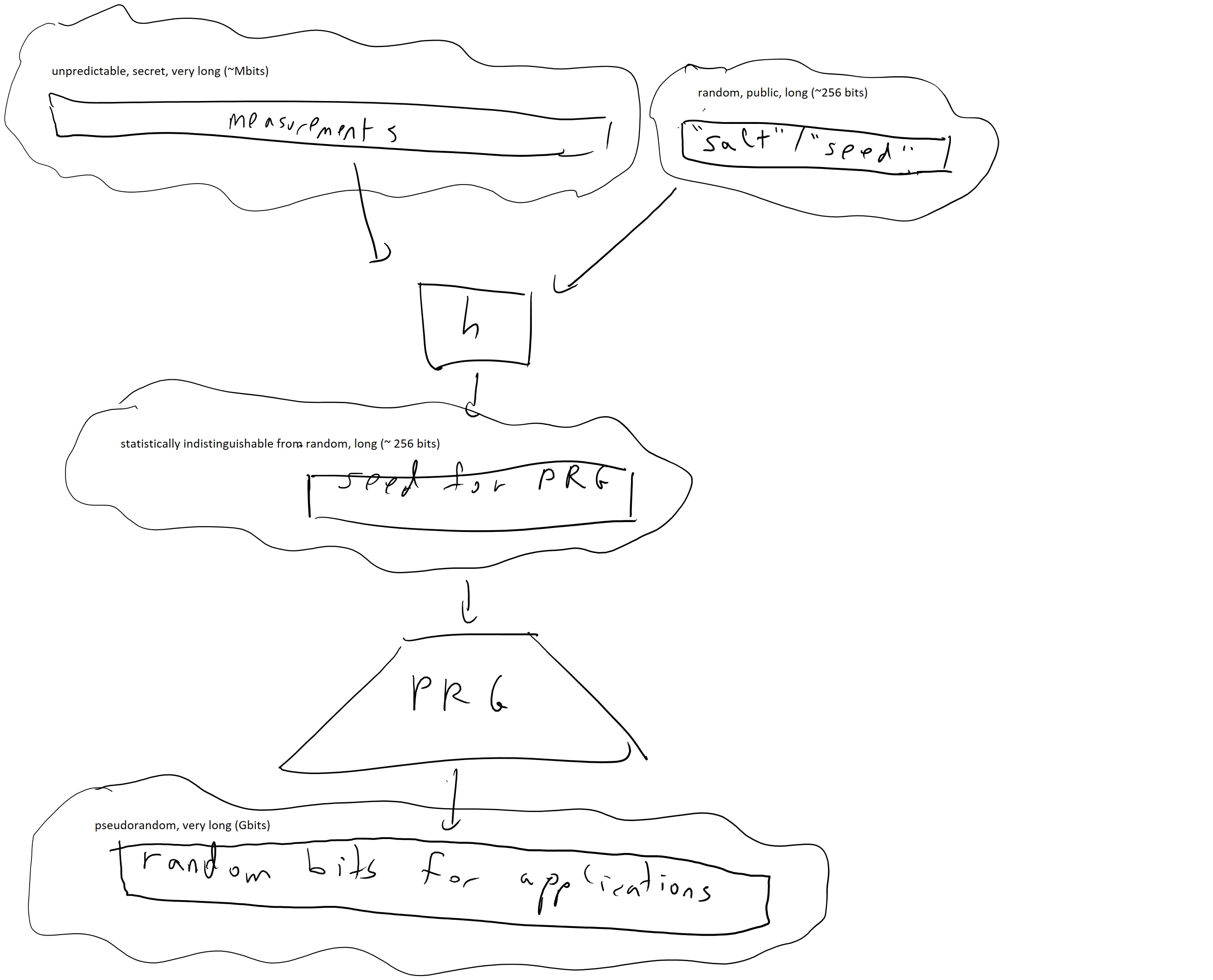
How do hash functions figure into this? The idea is that if an input \(x\) has \(n\) bits of entropy then \(h(x)\) would still have the same bits of entropy, as long as its output is larger than \(n\). In practice people use the notion of “entropy” in a rather loose sense, but we will try to be more precise below.

The entropy of a distribution \(D\) is meant to capture the amount of “uncertainty” you have over the distribution. The canonical example is when \(D\) is the uniform distribution over \(\{0,1\}^n\), in which case it has \(n\) bits of entropy. If you learn a single bit of \(D\) then you reduce the entropy by one bit. For example, if you learn that the \(17^{th}\) bit is equal to \(0\), then the new conditional distribution \(D'\) is the uniform distribution over all strings in \(x\in\{0,1\}^n\) such that \(x_{17}=0\) and has \(n-1\) bits of entropy. Entropy is invariant under permutations of the sample space, and only depends on the vector of probabilities, and thus for every set \(S\) all notions of entropy will give \(\log_2 |S|\) bits of entropy for the uniform distribution over \(S\). A distribution that is uniform over some set \(S\) is known as a flat distribution.

Where different notions of entropy begin to differ is when the distributions are not flat. The Shannon entropy follows the principle that “original uncertainty = knowledge learned + new uncertainty”. That is, it obeys the chain rule which is that if a random variable \((X,Y)\) has \(n\) bits of entropy, and \(X\) has \(k\) bits of entropy, then after learning \(X\) on average \(Y\) will have \(n-k\) bits of entropy. That is,

\(H_{Shannon}(X)+H_{Shannon}(Y|X) = H_{Shannon}(X,Y)\)

Where the entropy of a conditional distribution \(Y|X\) is simply \(\E_{x\leftarrow X} H_{Shannon}(Y|X=x)\) where \(Y|X=x\) is the distribution on \(Y\) obtained by conditioning on the event that \(X=x\).

If \((p_1,\ldots,p_m)\) is a vector of probabilities summing up to \(1\) and let us assume they are rounded so that for every \(i\), \(p_i = k_i/2^n\) for some integer \(k_i\). We can then split the set \(\{0,1\}^n\) into \(m\) disjoint sets \(S_1,\ldots,S_m\) where \(|S_i|=k_i\), and consider the probability distribution \((X,Y)\) where \(Y\) is uniform over \(\{0,1\}^n\), and \(X\) is equal to \(i\) whenever \(Y\in S_i\). Therefore, by the principles above we know that \(H_{Shannon}(X,Y)=n\) (since \(X\) is completely determined by \(Y\) and hence \((X,Y)\) is uniform over a set of \(2^n\) elements), and \(H(Y|X)= \E \log k_i\). Thus the chain rule tells us that \(H_{Shannon}(X) = H(X,Y) - H(Y|X) = n - \sum_{i=1}^m p_i \log(k_i) = n - \sum_{i=1}^m p_i \log(2^n p_i)\) since \(p_i = k_i/2^n\). Since \(\log(2^n p_i) = n + \log(p_i)\) we see that this means that

using the fact that \(\sum_i p_i = 1\).

The Shannon entropy has many attractive properties, but it turns out that for cryptographic applications, the notion of min entropy is more appropriate. For a distribution \(X\) the min-entropy is simply defined as \(H_{\infty}(X)= \min_x \log(1/\Pr[X=x])\).³ Note that if \(X\) is flat then \(H_{\infty}(X)=H_{Shannon}(X)\) and that \(H_{\infty}(X) \leq H_{Shannon}(X)\) for all \(X\). We can now formally define the notion of an extractor:

The idea is that we apply the hash function to our measurements in \(\{0,1\}^\ell\) then if those measurements had at least \(k\) bits of entropy (with some extra “security margin”) then the output \(h_s(X)\) will be as good as random. Since the “salt” value \(s\) is not secret, it can be chosen once at random and hardwired into the description of the function. (Indeed in practice people often do not explicitly use such a “salt”, but the hash function description contain some parameters IV that play a similar role.)

Forward and backward secrecy

A cryptographic tool such as encryption is clearly insecure if the adversary learns the private key, and similarly the output of a pseudorandom generator is insecure if the adversary learns the seed. So, it might seem as if it’s “game over” once this happens. However, there is still some hope. For example, if the adversary learns it at time \(t\) but didn’t know it before then, then one could hope that she does not learn the information that was exchanged up to time \(t-1\). This property is known as “forward secrecy”. It had recently gained interest as means to protect against powerful “attackers” such as the NSA that may record the communication transcripts in the hope of deciphering them in some future after it had learned the secret key. In the context of pseudorandom generators, one could hope for both forward and backward secrecy. Forward secrecy means that the state of the generator is updated at every point in time in a way that learning the state at time \(t\) does not help in recovering past state, and “backward secrecy” means that we can recover from the adversary knowing our internal state by updating the generator with fresh entropy. See this paper of me and Halevi for some discussions of this issue, as well as this later work by Dodis et al.

Comments

Comments are posted on the GitHub repository using the utteranc.es app. A GitHub login is required to comment. If you don't want to authorize the app to post on your behalf, you can also comment directly on the GitHub issue for this page.

Compiled on 11/17/2021 22:36:11

Copyright 2021, Boaz Barak.
This work is licensed under a Creative Commons Attribution-NonCommercial-NoDerivatives 4.0 International License.

Produced using pandoc and panflute with templates derived from gitbook and bookdown.