See any bugs/typos/confusing explanations? Open a GitHub issue. You can also comment below
★ See also the PDF version of this chapter (better formatting/references) ★
Computational Security
Additional reading: Sections 2.2 and 2.3 in Boneh-Shoup book. Chapter 3 up to and including Section 3.3 in Katz-Lindell book.
Recall our cast of characters- Alice and Bob want to communicate securely over a channel that is monitored by the nosy Eve. In the last lecture, we have seen the definition of perfect secrecy that guarantees that Eve cannot learn anything about their communication beyond what she already knew. However, this security came at a price. For every bit of communication, Alice and Bob have to exchange in advance a bit of a secret key. In fact, the proof of this result gives rise to the following simple Python program that can break every encryption scheme that uses, say, a \(128\) bit key, with a \(129\) bit message:
from itertools import product # Import an iterator for cartesian products
from random import choice # choose random element of list

# Gets ciphertext as input and two potential plaintexts
# Returns most likely plaintext
# We assume we have access to the function Encrypt(key,plaintext)
def Distinguish(ciphertext,plaintext1,plaintext2):
    for key in product([0,1], repeat = 128): # Iterate over all possible keys of length 128
        if Encrypt(key, plaintext1)==ciphertext:
            return plaintext1
        if Encrypt(key, plaintext2)==ciphertext:
            return plaintext2
    return choice([plaintext1,plaintext2])
The program Distinguish will break any \(128\)-bit key and \(129\)-bit message encryption Encrypt, in the sense that there exist a pair of messages \(m_0,m_1\) such that Distinguish\((\)Encrypt\((k,m_b),m_0,m_1)=m_b\) with probability at least \(0.75\) over \(k \leftarrow_R \{0,1\}^n\) and \(b \leftarrow_R \{0,1\}\).
Now, generating, distributing, and protecting huge keys causes immense logistical problems, which is why almost all encryption schemes used in practice do in fact utilize short keys (e.g., \(128\) bits long) with messages that can be much longer (sometimes even terabytes or more of data).
So, why can’t we use the above Python program to break all encryptions in the Internet and win infamy and fortune? We can in fact, but we’ll have to wait a really long time, since the loop in Distinguish will run \(2^{128}\) times, which will take much more than the lifetime of the universe to complete, even if we used all the computers on the planet.
However, the fact that this particular program is not a feasible attack, does not mean there does not exist a different attack. But this still suggests a tantalizing possibility: if we consider a relaxed version of perfect secrecy that restricts Eve to performing computations that can be done in this universe (e.g., less than \(2^{256}\) steps should be safe not just for human but for all potential alien civilizations) then can we bypass the impossibility result and allow the key to be much shorter than the message?
This in fact does seem to be the case, but as we’ve seen, defining security is a subtle task, and will take some care. As before, the way we avoid (at least some of) the pitfalls of so many cryptosystems in history is that we insist on very precisely defining what it means for a scheme to be secure.
Let us defer the discussion how one defines a function being computable in “less than \(T\) operations” and just say that there is a way to formally do so. We will want to say that a scheme has “\(256\) bits of security” if it is not possible to break it using less than \(2^{256}\) operations, and more generally that it has \(t\) bits of security if it can’t be broken using less than \(2^t\) operations. Given the perfect secrecy definition we saw last time, a natural attempt for defining computational secrecy would be the following:
An encryption scheme \((E,D)\) has \(t\) bits of computational secrecy if for every two distinct plaintexts \(\{m_0,m_1\} \subseteq {\{0,1\}}^\ell\) and every strategy of Eve using at most \(2^t\) computational steps, if we choose at random \(b\in{\{0,1\}}\) and a random key \(k\in{\{0,1\}}^n\), then the probability that Eve guesses \(m_b\) after seeing \(E_k(m_b)\) is at most \(1/2\).
Note: It is important to keep track of what is known and unknown to the adversary Eve. The adversary knows the set \(\{ m_0,m_1 \}\) of potential messages, and the ciphertext \(y=E_k(m_b)\). The only things she doesn’t know are whether \(b=0\) or \(b=1\), and the value of the secret key \(k\). In particular, because \(m_0\) and \(m_1\) are known to Eve, it does not matter whether we define Eve’s goal in this “security game” as outputting \(m_b\) or as outputting \(b\).
Definition 2.1 seems very natural, but is in fact impossible to achieve if the key is shorter than the message.
Before reading further, you might want to stop and think if you can prove that there is no, say, encryption scheme with \(\sqrt{n}\) bits of computational security satisfying Definition 2.1 with \(\ell = n+1\) and where the time to compute the encryption is polynomial.
The reason Definition 2.1 can’t be achieved is that if the message is even one bit longer than the key, we can always have a very efficient procedure that achieves success probability of about \(1/2 + 2^{-n-1}\) by guessing the key. This is because we can replace the loop in the Python program Distinguish by choosing the key at random. Since we have some small chance of guessing correctly, we will get a small advantage over half.
Of course an advantage of \(2^{-256}\) in guessing the message is not really something we would worry about. For example, since the earth is about 5 billion years old, we can estimate the chance that an asteroid of the magnitude that caused the dinosaurs’ extinction will hit us this very second to be about \(2^{-60}\). Hence we want to relax the notion of computational security so it would not consider guessing with such a tiny advantage as a “true break” of the scheme. The resulting definition is the following:
An encryption scheme \((E,D)\) has \(t\) bits of computational secrecy1 if for every two distinct plaintexts \(\{m_0,m_1\} \subseteq {\{0,1\}}^\ell\) and every strategy of Eve using at most \(2^t\) computational steps, if we choose at random \(b\in{\{0,1\}}\) and a random key \(k\in{\{0,1\}}^n\), then the probability that Eve guesses \(m_b\) after seeing \(E_k(m_b)\) is at most \(1/2+2^{-t}\).
Having learned our lesson, let’s try to see that this strategy does give us the kind of conditions we desired. In particular, let’s verify that this definition implies the analogous condition to perfect secrecy.
If \((E,D)\) has \(t\) bits of computational secrecy as per Definition 2.2 then for every subset \(M \subseteq {\{0,1\}}^\ell\) and every strategy of Eve using at most \(2^t-(100\ell+100)\) computational steps, if we choose at random \(m\in M\) and a random key \(k\in{\{0,1\}}^n\), then the probability that Eve guesses \(m\) after seeing \(E_k(m)\) is at most \(1/|M|+2^{-t+1}\).
Before proving this theorem note that it gives us a pretty strong guarantee. In the exercises we will strengthen it even further showing that no matter what prior information Eve had on the message before, she will never get any non-negligible new information on it.2 One way to phrase it is that if the sender used a \(256\)-bit secure encryption to encrypt a message, then your chances of getting to learn any additional information about it before the universe collapses are more or less the same as the chances that a fairy will materialize and whisper it in your ear.
Before reading the proof, try to again review the proof of Theorem 1.8, and see if you can generalize it yourself to the computational setting.
The proof is rather similar to the equivalence of guessing one of two messages vs. one of many messages for perfect secrecy (i.e., Theorem 1.8). However, in the computational context we need to be careful in keeping track of Eve’s running time. In the proof of Theorem 1.8 we showed that if there exists:
- A subset \(M\subseteq {\{0,1\}}^\ell\) of messages
and
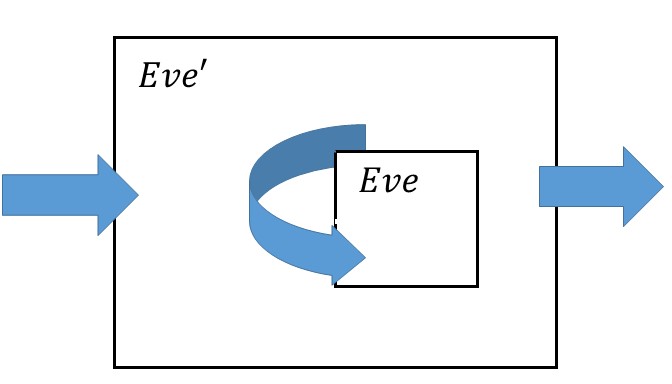
An adversary \(Eve:{\{0,1\}}^o\rightarrow{\{0,1\}}^\ell\) such that
\[ \Pr_{m{\leftarrow_{\tiny R}}M, k{\leftarrow_{\tiny R}}{\{0,1\}}^n}[ Eve(E_k(m))=m ] > 1/|M| \]
Then there exist two messages \(m_0,m_1\) and an adversary \(Eve':{\{0,1\}}^o\rightarrow{\{0,1\}}^\ell\) such that \(\Pr_{b{\leftarrow_{\tiny R}}{\{0,1\}},k{\leftarrow_{\tiny R}}{\{0,1\}}^n}[Eve'(E_k(m_b))=m_b ] > 1/2\).
To adapt this proof to the computational setting and complete the proof of the current theorem it suffices to show that:
If the probability of \(Eve\) succeeding was \(\tfrac{1}{|M|} + \epsilon\) then the probability of \(Eve'\) succeeding is at least \(\tfrac{1}{2} + \epsilon/2\).
If \(Eve\) can be computed in \(T\) operations, then \(Eve'\) can be computed in \(T + 100\ell + 100\) operations.
This will imply that if \(Eve\) ran in polynomial time and had polynomial advantage over \(1/|M|\) in guessing a plaintext chosen from \(M\), then \(Eve'\) would run in polynomial time and have polynomial advantage over \(1/2\) in guessing a plaintext chosen from \(\{ m_0,m_1\}\).
The first item can be shown by simply doing the same proof more carefully, keeping track how the advantage over \(\tfrac{1}{|M|}\) for \(Eve\) translates into an advantage over \(\tfrac{1}{2}\) for \(Eve'\). As the world’s most annoying saying goes, doing this is an excellent exercise for the reader.
The second item is obtained by looking at the definition of \(Eve'\) from that proof. On input \(c\), \(Eve'\) computed \(m=Eve(c)\) (which costs \(T\) operations), checked if \(m=m_0\) (which costs, say, at most \(5\ell\) operations), and then outputted either \(1\) or a random bit (which is a constant, say at most \(100\) operations).
Proof by reduction
The proof of Theorem 2.3 is a model to how a great many of the results in this course will look like. Generally we will have many theorems of the form:
“If there is a scheme \(S'\) satisfying security definition \(X'\) then there is a scheme \(S\) satisfying security definition \(X\)”
In the context of Theorem 2.3, \(X'\) was “having \(t\) bits of security” (in the context distinguishing between encryptions of two ciphertexts) and \(X\) was the more general notion of hardness of getting a non-trivial advantage over guessing for an encryption of a random \(m\in M\). While in Theorem 2.3 the encryption scheme \(S\) was the same as \(S'\), this need not always be the case. However, all of the proofs of such statements will have the same global structure— we will assume towards a contradiction, that there is an efficient adversary strategy \(Eve\) demonstrating that the scheme \(S\) violates the security notion \(X\), and build from \(Eve\) a strategy \(Eve'\) demonstrating that \(S'\) violates \(X'\). This is such an important point that it deserves repeating:
The way you show that if \(S'\) is secure then \(S\) is secure is by giving a transformation from an adversary that breaks \(S\) into an adversary that breaks \(S'\)
For computational secrecy, we will always want that \(Eve'\) will be efficient if \(Eve\) is, and that will usually be the case because \(Eve'\) will simply use \(Eve\) as a black box, which it will not invoke too many times, and addition will use some polynomial time preprocessing and postprocessing. The more challenging parts of such proofs are typically:
Coming up with the strategy \(Eve'\).
Analyzing the probability of success and in particular showing that if \(Eve\) had non-negligible advantage then so will \(Eve'\).
Note that, just like in the context of NP completeness or uncomputability reductions, security reductions work backwards. That is, we construct the scheme \(S\) based on the scheme \(S'\), but then prove that we can transform an algorithm breaking \(S\) into an algorithm breaking \(S'\). Just like in computational complexity, it can sometimes be hard to keep track of the direction of the reduction. In fact, cryptographic reductions can be even subtler, since they involve an interplay of several entities (for example, sender, receiver, and adversary) and probabilistic choices (e.g., over the message to be sent and the key).
The asymptotic approach
For practical security, often every bit of security matters. We want our keys to be as short as possible and our schemes to be as fast as possible while satisfying a particular level of security. In practice we would usually like to ensure that when we use a smallish security parameter such as \(n\) in the few hundreds or thousands then:
The honest parties (the parties running the encryption and decryption algorithms) are extremely efficient, something like 100-1000 cycles per byte of data processed. In theory terms we would want them be using an \(O(n)\) or at worst \(O(n^2)\) time algorithms with not-too-big hidden constants.
We want to protect against adversaries (the parties trying to break the encryption) that have much vaster computational capabilities. A typical modern encryption is built so that using standard key sizes it can withstand the combined computational powers of all computers on earth for several decades. In theory terms we would want the time to break the scheme to be \(2^{\Omega(n)}\) (or if not, at least \(2^{\Omega(\sqrt{n})}\) or \(2^{\Omega(n^{1/3})}\)) with not too small hidden constants.
For implementing cryptography in practice, the tradeoff between security and efficiency can be crucial. However, for understanding the principles behind cryptography, keeping track of concrete security can be a distraction, and so just like we do in algorithms courses, we will use asymptotic analysis (also known as big Oh notation) to sweep many of those details under the carpet.
To a first approximation, there will be only two types of running times we will encounter in this course:
Polynomial running time of the form \(d\cdot n^c\) for some constants \(d,c>0\) (or \(poly(n)=n^{O(1)}\) for short), which we will consider as efficient.
Exponential running time of the form \(2^{d\cdot n^{\epsilon}}\) for some constants \(d,\epsilon >0\) (or \(2^{n^{\Omega(1)}}\) for short) which we will consider as infeasible.3
Another way to say it is that in this course, if a scheme has any security at all, it will have at least \(n^{\epsilon}\) bits of security where \(n\) is the length of the key and \(\epsilon>0\) is some absolute constant such as \(\epsilon=1/3\). Hence in this course, whenever you hear the term “super polynomial”, you can equate it in your mind with “exponential” and you won’t be far off the truth.
These are not all the theoretically possible running times. One can have intermediate functions such as \(n^{\log n}\) though we will generally not encounter those. To make things clean (and to correspond to standard terminology), we will generally associate “efficient computation” with polynomial time in \(n\) where \(n\) is either its input length or the key size (the key size and input length will always be polynomially related, and so this choice won’t matter). We want our algorithms (encryption, decryption, etc.) to be computable in polynomial time, but to require super polynomial time to break.
Negligible probabilities. In cryptography, we care not just about the running time of the adversary but also about their probability of success (which should be as small as possible). If \(\mu:\N \rightarrow [0,\infty)\) is a function (which we’ll often think of as corresponding to the adversary’s probability of success or advantage over the trivial probability, as a function of the key size \(n\)) then we say that \(\mu(n)\) is negligible if it’s smaller than the inverse of every (positive) polynomial. Our security definitions will have the following form:
"Scheme \(S\) is secure if for every polynomial \(p(\cdot)\) and \(p(n)\) time adversary \(Eve\), there is some negligible function \(\mu\) such that the probability that \(Eve\) succeeds in the security game for \(S\) is at most \(trivial + \mu(n)\)"
We now make these notions more formal.
A function \(\mu:\mathbb{N} \rightarrow [0,\infty)\) is negligible if for every polynomial \(p:\N \rightarrow \N\) there exists \(N \in \N\) such that \(\mu(n) < \tfrac{1}{p(n)}\) for every \(n>N\).4
The following exercise provides a good way to get some comfort with this definition:
Let \(\mu:\N \rightarrow [0,\infty)\) be a negligible function. Prove that for every polynomials \(p,q:\R \rightarrow \R\) with non-negative coefficients such that \(p(0) = 0\), the function \(\mu':\N \rightarrow [0,\infty)\) defined as \(\mu'(n) = p(\mu(q(n)))\) is negligible.
Let \(\mu:\N \rightarrow [0,\infty)\). Prove that \(\mu\) is negligible if and only if for every constant \(c\), \(\lim_{n \rightarrow \infty} n^c \mu(n) = 0\).
The above definitions could be confusing if you haven’t encountered asymptotic analysis before. Reading the beginning of Chapter 3 (pages 43-51) in the KL book, as well as the mathematical background lecture in my intro to TCS notes can be extremely useful. As a rule of thumb, if every time you see the word “polynomial” you imagine the function \(n^{10}\) and every time you see the word “negligible” you imagine the function \(2^{-\sqrt{n}}\) then you will get the right intuition.
What you need to remember is that negligible is much smaller than any inverse polynomial, while polynomials are closed under multiplication, and so we have the “equations”
and
As mentioned, in practice people really want to get as close as possible to \(n\) bits of security with an \(n\) bit key, but we would be happy as long as the security grows with the key, so when we say a scheme is “secure” you can think of it having \(\sqrt{n}\) bits of security (though any function growing faster than \(\log n\) would be fine as well).
From now on, we will require all of our encryption schemes to be efficient which means that the encryption and decryption algorithms should run in polynomial time. Security will mean that any efficient adversary can make at most a negligible gain in the probability of guessing the message over its a priori probability.5
We can now formally define computational secrecy in asymptotic terms:
An encryption scheme \((E,D)\) is computationally secret if for every two distinct plaintexts \(\{m_0,m_1\} \subseteq {\{0,1\}}^\ell\) and every efficient (i.e., polynomial time) strategy of Eve, if we choose at random \(b\in{\{0,1\}}\) and a random key \(k\in{\{0,1\}}^n\), then the probability that Eve guesses \(m_b\) after seeing \(E_k(m_b)\) is at most \(1/2+\mu(n)\) for some negligible function \(\mu(\cdot)\).
Counting number of operations.
One more detail that we’ve so far ignored is what does it mean exactly for a function to be computable using at most \(T\) operations. Fortunately, when we don’t really care about the difference between \(T\) and, say, \(T^2\), then essentially every reasonable definition gives the same answer.6 Formally, we can use the notions of Turing machines, Boolean circuits, or straightline programs to define complexity. For concreteness, let’s define that a function \(F:{\{0,1\}}^n\rightarrow{\{0,1\}}^m\) has complexity at most \(T\) if there is a Boolean circuit that computes \(F\) using at most \(T\) Boolean gates (say AND/OR/NOT or NAND; alternatively you can choose your favorite universal gate sets.) We will often also consider probabilistic functions in which case we allow the circuit a RAND gate that outputs a single random bit (though this in general does not give extra power). The fact that we only care about asymptotics means you don’t really need to think of gates when arguing in cryptography. However, it is comforting to know that this notion has a precise mathematical formulation.
Uniform vs non-uniform models. While many computational texts focus on models such as Turing machines, in cryptography it is more convenient to use Boolean circuits which are a non uniform model of computation in the sense that we allow a different circuit for every given input length. The reasons are the following:
Circuits can express finite computation, while Turing machines only make sense for computing on arbitrarily large input lengths, and so we can make sense of notions such as “\(t\) bits of computational security”.
Circuits allow the notion of “hardwiring” whereby if we can compute a certain function \(F:\{0,1\}^{n+s} \rightarrow \{0,1\}^m\) using a circuit of \(T\) gates and have a string \(w \in \{0,1\}^s\) then we can compute the function \(x \mapsto F(xw)\) using \(T\) gates as well. This is useful in many cryptograhic proofs.
One can build the theory of cryptography using Turing machines as well, but it is more cumbersome.
Later on in the course, both our cryptographic schemes and the adversaries will extend beyond simple functions that map an input to an output, and we will consider interactive algorithms that exchange messages with one another. Such an algorithm can be implemented using circuits or Turing machines that take as input the prior state and the history of messages up to a certain point in the interaction, and output the next message in the interaction. The number of operations used in such a strategy is the total number of gates used in computing all the messages.
Our first conjecture
We are now ready to make our first conjecture:
The Cipher Conjecture:7 There exists a computationally secret encryption scheme \((E,D)\) (where \(E,D\) are efficient) with length function \(\ell(n)=n+1\).
A conjecture is a well defined mathematical statement which (1) we believe is true but (2) don’t know yet how to prove. Proving the cipher conjecture will be a great achievement and would in particular settle the P vs NP question, which is arguably the fundamental question of computer science. That is, the following theorem is known:
If \(P=\ensuremath{\mathit{NP}}\) then there does not exist a computationally secret encryption with efficient \(E\) and \(D\) and where the message is longer than the key.
We just sketch the proof, as this is not the focus of this course. If \(P=\ensuremath{\mathit{NP}}\) then whenever we have a loop that searches through some domain to find some string that satisfies a particular property (like the loop in the Distinguish subroutine above that searches over all keys) then this loop can be sped up exponentially .
While it is very widely believed that \(P\neq \ensuremath{\mathit{NP}}\), at the moment we do not know how to prove this, and so have to settle for accepting the cipher conjecture as essentially an axiom, though we will see later in this course that we can show it follows from some seemingly weaker conjectures.
There are several reasons to believe the cipher conjecture. We now briefly mention some of them:
Intuition: If the cipher conjecture is false then it means that for every possible cipher we can make the exponential time attack described above become efficient. It seems “too good to be true” in a similar way that the assumption that P=NP seems too good to be true.
Concrete candidates: As we will see in the next lecture, there are several concrete candidate ciphers using keys shorter than messages for which despite tons of effort, no one knows how to break them. Some of them are widely used and hence governments and other benign or not so benign organizations have every reason to invest huge resources in trying to break them. Despite that as far as we know (and we know a little more after Edward Snowden’s revelations) there is no significant break known for the most popular ciphers. Moreover, there are other ciphers that can be based on canonical mathematical problems such as factoring large integers or decoding random linear codes that are immensely interesting in their own right, independently of their cryptographic applications.
Minimalism: Clearly if the cipher conjecture is false then we also don’t have a secure encryption with a message, say, twice as long as the key. But it turns out the cipher conjecture is in fact necessary for essentially every cryptographic primitive, including not just private key and public key encryptions but also digital signatures, hash functions, pseudorandom generators, and more. That is, if the cipher conjecture is false then to a large extent cryptography does not exist, and so we essentially have to assume this conjecture if we want to do any kind of cryptography.
Why care about the cipher conjecture?
“Give me a place to stand, and I shall move the world” Archimedes, circa 250 BC
Every perfectly secure encryption scheme is clearly also computationally secret, and so if we required a message of size \(n\) instead \(n+1\), then the conjecture would have been trivially satisfied by the one-time pad. However, having a message longer than the key by just a single bit does not seem that impressive. Sure, if we used such a scheme with \(128\)-bit long keys, our communication will be smaller by a factor of \(128/129\) (or a saving of about \(0.8\%\)) over the one-time pad, but this doesn’t seem worth the risk of using an unproven conjecture. However, it turns out that if we assume this rather weak condition, we can actually get a computationally secret encryption scheme with a message of size \(p(n)\) for every polynomial \(p(\cdot)\). In essence, we can fix a single \(n\)-bit long key and communicate securely as many bits as we want!
Moreover, this is just the beginning. There is a huge range of other useful cryptographic tools that we can obtain from this seemingly innocent conjecture: (We will see what all these names and some of these reductions mean later in the course.)
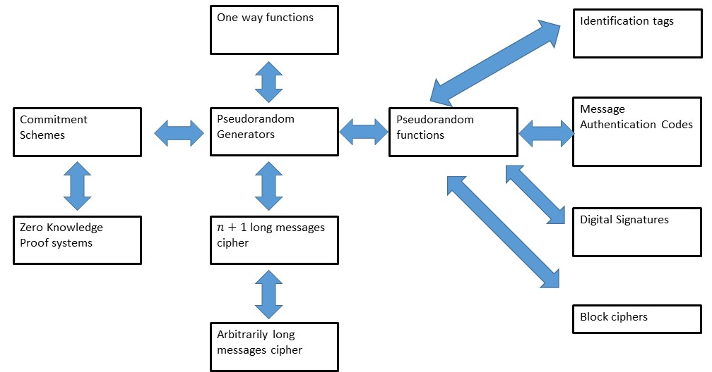
We will soon see the first of the many reductions we’ll learn in this course. Together this “web of reductions” forms the scientific core of cryptography, connecting many of the core concepts and enabling us to construct increasingly sophisticated tools based on relatively simple “axioms” such as the cipher conjecture.
Prelude: Computational Indistinguishability
The task of Eve in breaking an encryption scheme is to distinguish between an encryption of \(m_0\) and an encryption of \(m_1\). It turns out to be useful to consider this question of when two distributions are computationally indistinguishable more broadly:
Let \(X\) and \(Y\) be two distributions over \({\{0,1\}}^m\). We say that \(X\) and \(Y\) are \((T,\epsilon)\)-computationally indistinguishable, denoted by \(X \approx_{T,\epsilon} Y\), if for every function \(D:\{0,1\}^m \rightarrow \{0,1\}\) computable with at most \(T\) operations,
Prove that for every \(X,Y\) and \(T,\epsilon\) as above \(X \approx_{T,\epsilon} Y\) if and only if for every \(\leq T\)-operation computable \(Eve\), the probability that \(Eve\) wins in the following game is at most \(1/2 + \epsilon/2\):
We pick \(b \leftarrow_R \{0,1\}\).
If \(b=0\), we let \(w \leftarrow_R X\). If \(b=1\), we let \(w \leftarrow_R Y\).
We give \(Eve\) the input \(w\), and \(Eve\) outputs \(b' \in \{0,1\}\).
\(Eve\) wins if \(b=b'\).
Working out this exercise on your own is a great way to get comfortable with computational indistinguishability, which is a fundamental notion.
For every function \(Eve:\{0,1\}^m \rightarrow \{0,1\}\), let \(p_X = \Pr[ Eve(X)=1]\) and \(p_Y = \Pr[Eve(Y)=1]\).
Then the probability that \(Eve\) wins the game is:
and since \(\Pr[b=0]=\Pr[b=1]=1/2\) this is
We see that \(Eve\) wins the game with success \(1/2 + \epsilon/2\) if and only if
For the other direction, assume that \(X\) and \(Y\) are not computationally indistinguishable and let \(Eve\) be a \(T\) time operation function such that
Then by definition of absolute value, there are two options. Either \(\Pr[ Eve(X) = 1 ] - \Pr[Eve(Y)=1] \geq \epsilon\) in which case \(Eve\) wins the game with probability at least \(1/2 + \epsilon/2\). Otherwise \(\Pr[ Eve(X) = 1 ] - \Pr[Eve(Y)=1] \leq -\epsilon\), in which case the function \(Eve'(w)=1-Eve(w)\) (which is just as easy to compute) wins the game with probability at least \(1/2 + \epsilon/2\).
Note that above we assume that the class of “functions computable in at most \(T\) operations” is closed under negation, in the sense that if \(F\) is in this class, then \(1-F\) is also. For standard Boolean circuits, this can be done if we don’t count negation gates (which can change the total circuit size by at most a factor of two), or we can allow for \(Eve'\) to require a constant additional number of operations, in which case the exercise is still essentially true but is slightly more cumbersome to state.
As we did with computational secrecy, we can also define an asymptotic definition of computational indistinguishability.
Let \(m:\N \rightarrow \N\) be some function and let \(\{ X_n \}_{n\in \N}\) and \(\{ Y_n \}_{n\in \N}\) be two sequences of distributions such that \(X_n\) and \(Y_n\) are distributions over \(\{0,1\}^{m(n)}\).
We say that \(\{ X_n \}_{n\in \N}\) and \(\{ Y_n \}_{n\in\N}\) are computationally indistinguishable, denoted by \(\{ X_n \}_{n\in\N} \approx \{ Y_n \}_{n\in\N}\), if for every polynomial \(p:\N \rightarrow \N\) and sufficiently large \(n\), \(X_n \approx_{p(n), 1/p(n)} Y_n\).
Solving the following asymptotic analog of Solved Exercise 2.1 is a good way to get comfortable with the asymptotic definition of computational indistinguishability:
Let \(\{ X_n \}_{n\in \N},\{Y_n\}_{n\in \N}\) and \(m:\N \rightarrow \N\) be as above. Then \(\{ X_n \}_{n\in\N} \approx \{ Y_n \}_{n\in\N}\) if and only if for every polynomial-time \(Eve\), there is some negligible function \(\mu\) such that \(Eve\) wins the following game with probability at most \(1/2 + \mu(n)\):
We pick \(b \leftarrow_R \{0,1\}\).
If \(b=0\), we let \(w \leftarrow_R X_n\). If \(b=1\), we let \(w \leftarrow_R Y_n\).
We give \(Eve\) the input \(w\), and \(Eve\) outputs \(b' \in \{0,1\}\).
\(Eve\) wins if \(b=b'\).
Dropping the index \(n\). Since the index \(n\) of our distributions would often be clear from context (indeed in most cases it will be the length of the key), we will sometimes drop it from our notation. So if \(X\) and \(Y\) are two random variables that depend on some index \(n\), we will say that \(X\) is computationally indistinguishable from \(Y\) (denoted as \(X \approx Y\)) when the sequences \(\{ X_n \}_{n\in \N}\) and \(\{ Y_n \}_{n\in\N}\) are computationally indistinguishable.
We can use computational indistinguishability to phrase the definition of computational secrecy more succinctly:
Let \((E,D)\) be a valid encryption scheme. Then \((E,D)\) is computationally secret if and only if for every two messages \(m_0,m_1 \in \{0,1\}^\ell\),
Working out the proof is an excellent way to make sure you understand both the definition of computational secrecy and computational indistinguishability, and hence we leave it as an exercise.
One intuition for computational indistinguishability is that it is related to some notion of distance. If two distributions are computationally indistinguishable, then we can think of them as “very close” to one another, at least as far as efficient observers are concerned. Intuitively, if \(X\) is close to \(Y\) and \(Y\) is close to \(Z\) then \(X\) should be close to \(Z\).8 Similarly if four distributions \(X,X',Y,Y'\) satisfy that \(X\) is close to \(Y\) and \(X'\) is close to \(Y'\), then you might expect that the distribution \((X,X')\) where we take two independent samples from \(X\) and \(X'\) respectively, is close to the distribution \((Y,Y')\) where we take two independent samples from \(Y\) and \(Y'\) respectively. We will now verify that these intuitions are in fact correct:
Suppose \(X_1 \approx_{T,\epsilon} X_2 \approx_{T,\epsilon} \cdots \approx_{T,\epsilon} X_m\). Then \(X_1 \approx_{T, (m-1)\epsilon} X_m\).
Suppose that there exists a \(T\) time \(Eve\) such that
Write
Thus,
Suppose that \(X_1,\ldots,X_\ell,Y_1,\ldots,Y_\ell\) are distributions over \({\{0,1\}}^n\) such that \(X_i \approx_{T,\epsilon} Y_i\). Then \((X_1,\ldots,X_\ell) \approx_{T-10\ell n,\ell\epsilon} (Y_1,\ldots,Y_\ell)\).
For every \(i\in\{0,\ldots,\ell\}\) we define \(H_i\) to be the distribution \((X_1,\ldots,X_i,Y_{i+1},\ldots,Y_\ell)\). Clearly \(H_\ell = (X_1,\ldots,X_\ell)\) and \(H_0 = (Y_1,\ldots,Y_\ell)\). We will prove that for every \(i\), \(H_{i-1} \approx_{T-10\ell n,\epsilon} H_i\), and the proof will then follow from the triangle inequality (can you see why?). Indeed, suppose towards the sake of contradiction that there was some \(i\in \{1,\ldots,\ell\}\) and some \(T-10\ell n\)-time \(Eve':{\{0,1\}}^{n\ell}\rightarrow{\{0,1\}}\) such that
In other words
By linearity of expectation we can write the difference of these two expectations as
By the averaging principle9 this means that there exist some values \(x_1,\ldots,x_{i-1},y_{i+1},\ldots,y_\ell\) such that
The above proof illustrates a powerful technique known as the hybrid argument whereby we show that two distribution \(C^0\) and \(C^1\) are close to each other by coming up with a sequence of distributions \(H_0,\ldots,H_t\) such that \(H_t = C^1, H_0 = C^0\), and we can argue that \(H_i\) is close to \(H_{i+1}\) for all \(i\). This type of argument repeats itself time and again in cryptography, and so it is important to get comfortable with it.
The Length Extension Theorem or Stream Ciphers
We now turn to show the length extension theorem, stating that if we have an encryption for \(n+1\)-length messages with \(n\)-length keys, then we can obtain an encryption with \(p(n)\)-length messages for every polynomial \(p(n)\). For a warm-up, let’s show the easier fact that we can transform an encryption such as above, into one that has keys of length \(tn\) and messages of length \(t(n+1)\) for every integer \(t\):
Suppose that \((E',D')\) is a computationally secret encryption scheme with \(n\) bit keys and \(n+1\) bit messages. Then the scheme \((E,D)\) where \(E_{k_1,\ldots,k_t}(m_1,\ldots,m_t)= (E'_{k_1}(m_1),\ldots, E'_{k_t}(m_t))\) and \(D_{k_1,\ldots,k_t}(c_1,\ldots,c_t)= (D'_{k_1}(c_1),\ldots, D'_{k_t}(c_t))\) is a computationally secret scheme with \(tn\) bit keys and \(t(n+1)\) bit messages.
This might seem “obvious” but in cryptography, even obvious facts are sometimes wrong, so it’s important to prove this formally. Luckily, this is a fairly straightforward implication of the fact that computational indisinguishability is preserved under many samples. That is, by the security of \((E',D')\) we know that for every two messages \(m,m' \in {\{0,1\}}^{n+1}\), \(E'_k(m) \approx E'_k(m')\) where \(k\) is chosen from the distribution \(U_n\). Therefore by the indistinguishability of many samples lemma, for every two tuples \(m_1,\ldots,m_t \in {\{0,1\}}^{n+1}\) and \(m'_1,\ldots,m'_t\in {\{0,1\}}^{n+1}\),
for random \(k_1,\ldots,k_t\) chosen independently from \(U_n\) which is exactly the condition that \((E,D)\) is computationally secret.
Randomized encryption scheme. We can now prove the full length extension theorem. Before doing so, we will need to generalize the notion of an encryption scheme to allow a randomized encryption scheme. That is, we will consider encryption schemes where the encryption algorithm can “toss coins” in its computation. There is a crucial difference between key material and such “as hoc” (sometimes also known as “ephemeral”) randomness. Keys need to be not only chosen at random, but also shared in advance between the sender and receiver, and stored securely throughout their lifetime. The “coin tosses” used by a randomized encryption scheme are generated “on the fly” and are not known to the receiver, nor do they need to be stored long term by the sender. So, allowing such randomized encryption does not make a difference for most applications of encryption schemes. In fact, as we will see later in this course, randomized encryption is necessary for security against more sophisticated attacks such as chosen plaintext and chosen ciphertext attacks, as well as for obtaining secure public key encryptions. We will use the notation \(E_k(m;r)\) to denote the output of the encryption algorithm on key \(k\), message \(m\) and using internal randomness \(r\). We often suppress the notation for the randomness, and hence use \(E_k(m)\) to denote the random variable obtained by sampling a random \(r\) and outputting \(E_k(m;r)\).
We can now show that given an encryption scheme with messages one bit longer than the key, we can obtain a (randomized) encryption scheme with arbitrarily long messages:
Suppose that there exists a computationally secret encryption scheme \((E',D')\) with key length \(n\) and message length \(n+1\). Then for every polynomial \(t(n)\) there exists a (randomized) computationally secret encryption scheme \((E,D)\) with key length \(n\) and message length \(t(n)\).
This is perhaps our first example of a non trivial cryptographic theorem, and the blueprint for this proof will be one that we will follow time and again during this course. Please make sure you read this proof carefully and follow the argument.
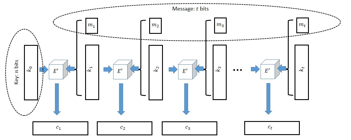
The construction, depicted in Figure 2.3, is actually quite natural and variants of it are used in practice for stream ciphers, which are ways to encrypt arbitrarily long messages using a fixed size key. The idea is that we use a key \(k_0\) of size \(n\) to encrypt (1) a fresh key \(k_1\) of size \(n\) and (2) one bit of the message. Now we can encrypt \(k_2\) using \(k_1\) and so on and so forth. We now describe the construction and analysis in detail.
Let \(t=t(n)\). We are given a cipher \(E'\) which can encrypt \(n+1\)-bit long messages with an \(n\)-bit long key and we need to encrypt a \(t\)-bit long message \(m=(m_1,\ldots,m_t) \in {\{0,1\}}^t\). Our idea is simple (at least in hindsight). Let \(k_0 {\leftarrow_{\tiny R}}{\{0,1\}}^n\) be our key (which is chosen at random). To encrypt \(m\) using \(k_0\), the encryption function will choose \(t\) random strings \(k_1,\ldots, k_t {\leftarrow_{\tiny R}}{\{0,1\}}^n\). We will then encrypt the \(n+1\)-bit long message \((k_1,m_1)\) with the key \(k_0\) to obtain the ciphertext \(c_1\), then encrypt the \(n+1\)-bit long message \((k_2,m_2)\) with the key \(k_1\) to obtain the ciphertext \(c_2\), and so on and so forth until we encrypt the message \((k_t,m_t)\) with the key \(k_{t-1}\).11 We output \((c_1,\ldots,c_t)\) as the final ciphertext.12
To decrypt \((c_1,\ldots,c_t)\) using the key \(k_0\), first decrypt \(c_1\) to learn \((k_1,m_1)\), then use \(k_1\) to decrypt \(c_2\) to learn \((k_2,m_2)\), and so on until we use \(k_{t-1}\) to decrypt \(c_t\) and learn \((k_t,m_t)\). Finally we can simply output \((m_1,\ldots,m_t)\).
The above are clearly valid encryption and decryption algorithms, and hence the real question becomes is it secure??. The intuition is that \(c_1\) hides all information about \((k_1,m_1)\) and so in particular the first bit of the message is encrypted securely, and \(k_1\) still can be treated as an unknown random string even to an adversary that saw \(c_1\). Thus, we can think of \(k_1\) as a random secret key for the encryption \(c_2\), and hence the second bit of the message is encrypted securely, and so on and so forth.
Our discussion above looks like a reasonable intuitive argument, but to make sure it’s true we need to give an actual proof. Let \(m,m' \in {\{0,1\}}^t\) be two messages. We need to show that \(E_{U_n}(m) \approx E_{U_n}(m')\). The heart of the proof will be the following claim:
Claim: Let \(\hat{E}\) be the algorithm that on input a message \(m\) and key \(k_0\) works like \(E\) except that its \(i^{th}\) block contains \(E'_{k_{i-1}}(k'_i,m_i)\) where \(k'_i\) is a random string in \({\{0,1\}}^n\), that is chosen independently of everything else including the key \(k_i\). Then, for every message \(m\in{\{0,1\}}^t\)
Note that \(\hat{E}\) is not a valid encryption scheme since it’s not at all clear there is a decryption algorithm for it. It is just an hypothetical tool we use for the proof. Since both \(E\) and \(\hat{E}\) are randomized encryption schemes (with \(E\) using \((t-1)n\) bits of randomness for the ephemeral keys \(k_1,\ldots,k_{t-1}\) and \(\hat{E}\) using \((2t-1)n\) bits of randomness for the ephemeral keys \(k_1,\ldots,k_t,k'_2,\ldots,k'_t\)), we can also write Equation 2.1 as
Once we prove the claim then we are done since we know that for every pair of messages \(m,m'\), \(E_{U_n}(m) \approx \hat{E}_{U_n}(m)\) and \(E_{U_n}(m') \approx \hat{E}_{U_n}(m')\) but \(\hat{E}_{U_n}(m) \approx \hat{E}_{U_n}(m')\) since \(\hat{E}\) is essentially the same as the \(t\)-times repetition scheme we analyzed above. Thus by the triangle inequality we can conclude that \(E_{U_n}(m) \approx E_{U_n}(m')\) as we desired.
Proof of claim: We prove the claim by the hybrid method. For \(j\in \{0,\ldots, t\}\), let \(H_j\) be the distribution of ciphertexts where in the first \(j\) blocks we act like \(\hat{E}\) and in the last \(t-j\) blocks we act like \(E\). That is, we choose \(k_0,\ldots,k_t,k'_1,\ldots,k'_t\) independently at random from \(U_n\) and the \(i^{th}\) block of \(H_j\) is equal to \(E'_{k_{i-1}}(k_i,m_i)\) if \(i>j\) and is equal to \(E'_{k_{i-1}}(k'_i,m_i)\) if \(i\leq j\). Clearly, \(H_t = \hat{E}_{U_n}(m)\) and \(H_0 = E_{U_n}(m)\) and so it suffices to prove that for every \(j\), \(H_{j-1} \approx H_j\). Indeed, let \(j \in \{1,\ldots,t\}\) and suppose towards the sake of contradiction that there exists an efficient \(Eve'\) such that
where \(\epsilon = \epsilon(n)\) is noticeable. By the averaging principle, there exists some fixed choice for \(k'_1,\ldots,k'_t,k_0,\ldots,k_{j-2},k_j,\ldots,k_t\) such that \((*)\) still holds. Note that in this case the only randomness is the choice of \(k_{j-1}{\leftarrow_{\tiny R}}U_n\) and moreover the first \(j-1\) blocks and the last \(t-j\) blocks of \(H_{j-1}\) and \(H_j\) would be identical and we can denote them by \(\alpha\) and \(\beta\) respectively and hence write \((*)\) as
But now consider the adversary \(Eve\) that is defined as \(Eve(c) = Eve'(\alpha,c,\beta)\). Then \(Eve\) is also efficient and by \((**)\) it can distinguish between \(E'_{U_n}(k_j,m_j)\) and \(E'_{U_n}(k'_j,m_j)\) thus contradicting the security of \((E',D')\). This concludes the proof of the claim and hence the theorem.
Appendix: The computational model
For concreteness sake let us give a precise definition of what it means for a function or probabilistic process \(f\) mapping \(\{0,1\}^n\) to \(\{0,1\}^m\) to be computable using \(T\) operations.
If you have taken any course on computational complexity (such as Harvard CS 121), then this is the model of Boolean circuits, except that we also allow randomization.
If you have not taken such a course, you might simply take it on faith that it is possible to model what it means for an algorithm to be able to map an input \(x\) into an output \(f(x)\) using \(T\) “elementary operations”.
In both cases you might want to skip this appendix and only return to it if you find something confusing.
The model we use is a Boolean circuit that also has a \(\ensuremath{\mathit{RAND}}\) gate that outputs a random bit. We could use as the basic set of gates the standard \(\ensuremath{\mathit{AND}}\), \(\ensuremath{\mathit{OR}}\) and \(\ensuremath{\mathit{NOT}}\) but for simplicity we use the one-element set \(\ensuremath{\mathit{NAND}}\). We represent the circuit as a straightline program, but this is of course just a matter of convenience. As shown (for example) in the CS 121 textbook, these two representations are identical.
A probabilistic straightline program consists of a sequence of lines, each one of them one of the following forms:
foo = NAND(bar, baz)wherefoo,bar,bazare variable identifiers.foo = RAND()wherefoois a variable identifier.
Given a program \(\pi\), we say that its size is the number of lines it contains. Variables of the form X[\(i\)] or Y[\(j\)] are considered input and output variables respectively. If the input variables range from \(0\) to \(n-1\) and the output variables range from \(0\) to \(m-1\) then the program computes the probabilistic process that maps \(\{0,1\}^n\) to \(\{0,1\}^m\) in the natural way. If \(F\) is a (probabilistic or deterministic) map of \(\{0,1\}^n\) to \(\{0,1\}^m\), the complexity of \(F\) is the size of the smallest program \(P\) that computes it.
If you haven’t taken a class such as CS121 before, you might wonder how such a simple model captures complicated programs that use loops, conditionals, and more complex data types than simply a bit in \(\{0,1\}\), not to mention some special purpose crypto-breaking devices that might involve tailor-made hardware. It turns out that it does (for the same reason we can compile complicated programming languages to run on silicon chips with a very limited instruction set). In fact, as far as we know, this model can capture even computations that happen in nature, whether it’s in a bee colony or the human brain (which contains about \(10^{10}\) neurons, so should in principle be simulatable by a program that has up to a few order of magnitudes of the same number of lines). Crucially, for cryptography, we care about such programs not because we want to actually run them, but because we want to argue about their non existence. If we have a process that cannot be computed by a straightline program of length shorter than \(2^{128}>10^{38}\) then it seems safe to say that a computer the size of the human brain (or even all the human and nonhuman brains on this planet) will not be able to perform it either.
Advanced note: non uniformity. The computational model we use in this class is non uniform (corresponding to Boolean circuits) as opposed to uniform (corresponding to Turing machines). If this distinction doesn’t mean anything to you, you can ignore it as it won’t play a significant role in what we do next. It basically means that we do allow our programs to have hardwired constants of \(poly(n)\) bits where \(n\) is the input/key length. In fact, to be precise, we will hold ourselves to a higher standard than our adversary, in the sense that we require our algorithms to be efficient in the stronger sense of being computable in uniform probabilistic polynomial time (for some fixed polynomial, often \(O(n)\) or \(O(n^2\))), while the adversary is allowed to use non uniformity.
Quantum computing. An interesting potential exception to this principle that every natural process should be simulatable by a straightline program of comparable complexity are processes where the quantum mechanical notions of interference and entanglement play a significant role. We will talk about this notion of quantum computing towards the end of the course, though note that much of what we say does not really change when we add quantum into the picture. As discussed in the CS 121 text, we can still capture these processes by straightline programs (that now have somewhat more complex form), and so most of what we’ll do just carries over in the same way to the quantum realm as long as we are fine with conjecturing the strong form of the cipher conjecture, namely that the cipher is infeasible to break even for quantum computers. All current evidence points toward this strong form being true as well. The field of constructing encryption schemes that are potentially secure against quantum computers is known as post quantum cryptography and we will return to this later in the course.
- ↩
Another version of “\(t\) bits of security” is that a scheme has \(t\) bits of security if for every \(t_1+t_2 \leq t\), an attacker running in \(2^{t_1}\) time can’t get success probability advantage more than \(2^{-t_2}\). However these two definitions only differ from one another by at most a factor of two. This may be important for practical applications (where the difference between \(64\) and \(32\) bits of security could be crucial) but won’t matter for our concerns.
- ↩
The latter property is known as “semantic security”, see also section 3.2.2 of Katz Lindell on “semantic security” and Section 2 of Boneh-Shoup “computational ciphers and semantic security”.
- ↩
Some texts reserve the term exponential to functions of the form \(2^{\epsilon n}\) for some \(\epsilon > 0\) and call a function such as, say, \(2^{\sqrt{n}}\) subexponential . However, we will generally not make this distinction in this course.
- ↩
Negligible functions are sometimes defined with image equalling \([0,1]\) as opposed to the set \([0,\infty)\) of non-negative real numbers, since they are typically used to bound probabilities. However, this does not make much difference since if \(\mu\) is negligible then for large enough \(n\), \(\mu(n)\) will be smaller than one.
- ↩
Note that there is a subtle issue here with the order of quantifiers. For a scheme to be efficient, the algorithms such as encryption and decryption need to run in some fixed polynomial time such as \(n^2\) or \(n^3\). In contrast we allow the adversary to run in any polynomial time. That is, for every \(c\), if \(n\) is large enough, then the scheme should be secure against an adversary that runs in time \(n^c\). This is in line with the general principle in cryptography that we always allow the adversary potentially much more resources than those used by the honest users. In practical security we often assume that the gap between the honest use and the adversary resources can be exponential. For example, a low power embedded device can encrypt messages that, as far as we know, are undecipherable even by a nation-state using super-computers and massive data centers.
- ↩
With some caveats that need to be added due to quantum computers: we’ll get to those later in the course, though they won’t change most of our theory. See also this discussion in my intro TCS textbook and this presentation of Aaronson on the “extended Church Turing thesis”.
- ↩
As will be the case for other conjectures we talk about, the name “The Cipher Conjecture” is not a standard name, but rather one we’ll use in this course. In the literature this conjecture is mostly referred to as the conjecture of existence of one way functions, a notion we will learn about later. These two conjectures a priori seem quite different but have been shown to be equivalent.
- ↩
Results of this form are known as “triangle inequalities” since they can be viewed as generalizations of the statement that for every three points on the plane \(x,y,z\), the distance from \(x\) to \(z\) is not larger than the distance from \(x\) to \(y\) plus the distance from \(y\) to \(z\). In other words, the edge \(\overline{x,z}\) of the triangle \((x,y,z)\) is not longer than the sum of the lengths of the other two edges \(\overline{x,y}\) and \(\overline{y,z}\).
- ↩
This is the principle that if the average grade in an exam was at least \(\alpha\) then someone must have gotten at least \(\alpha\), or in other words that if a real-valued random variable \(Z\) satisfies \({\mathbb{E}}[Z] \geq \alpha\) then \(\Pr[Z\geq \alpha]>0\).
- ↩
The cost \(10 \ell n\) is for the operations of feeding the “hardwired” strings \(x_1,\ldots,x_{i-1}\), \(y_{i+1},\ldots,y_\ell\) into \(Eve'\). These take up at most \(\ell n\) bits, and depending on the computational model, storing and feeding them into \(Eve'\) may take \(c\ell n\) steps for some small constant \(c<10\). In the future, we will usually ignore such minor details and simply say that if \(Eve'\) runs in polynomial time then so will \(Eve\).
- ↩
The keys \(k_1,\ldots,k_t\) are sometimes known as ephemeral keys in the crypto literature, since they are created only for the purposes of this particular interaction.
- ↩
The astute reader might note that the key \(k_t\) is actually not used anywhere in the encryption nor decryption and hence we could encrypt \(n\) more bits of the message instead in this final round. We used the current description for the sake of symmetry and simplicity of exposition.
Comments
Comments are posted on the GitHub repository using the utteranc.es app. A GitHub login is required to comment. If you don't want to authorize the app to post on your behalf, you can also comment directly on the GitHub issue for this page.
Compiled on 11/17/2021 22:36:25
Copyright 2021, Boaz Barak.

This work is
licensed under a Creative Commons
Attribution-NonCommercial-NoDerivatives 4.0 International License.
Produced using pandoc and panflute with templates derived from gitbook and bookdown.