See any bugs/typos/confusing explanations? Open a GitHub issue. You can also comment below
★ See also the PDF version of this chapter (better formatting/references) ★
Fully homomorphic encryption: Introduction and bootstrapping
In today’s era of “cloud computing”, much of individuals’ and businesses’ data is stored and computed on by third parties such as Google, Microsoft, Apple, Amazon, Facebook, Dropbox and many others. Classically, cryptography provided solutions to protecting data in motion from point A to point B. But these are not always sufficient to protect data at rest and particularly data in use. For example, suppose that Alice has some data \(x \in \{0,1\}^n\) (in modern applications \(x\) would well be terabytes in length or larger) that she wishes to store with the cloud service Bob, but is afraid that Bob will be hacked, subpoenaed or simply does not completely trust Bob.
Encryption does not seem to immediately solve the problem. Alice could store at Bob an encrypted version of the data and keep the secret key for herself. But then she would be at a loss if she wanted to do anything more with the data other than retrieving particular blocks of it. If she wanted to outsource computation to Bob as well, and compute \(f(x)\) for some function \(f\), then she would need to share the secret key with Bob, thus defeating the purpose of encrypting the data in the first place.
For example, after the computing systems of Office of Personell Management (OPM) were discovered to be hacked in June of 2015, revealing sensitive information, including fingerprints and all data gathered during security clearance checks of up to 18 million people, DHS assistant secretary for cybersecurity and communications Andy Ozment said that encryption wouldn’t have helped preventing it since “if an adversary has the credentials of a user on the network, then they can access data even if it’s encrypted, just as the users on the network have to access data”. So, can we encrypt data in a way that still allows some access and computing on it?
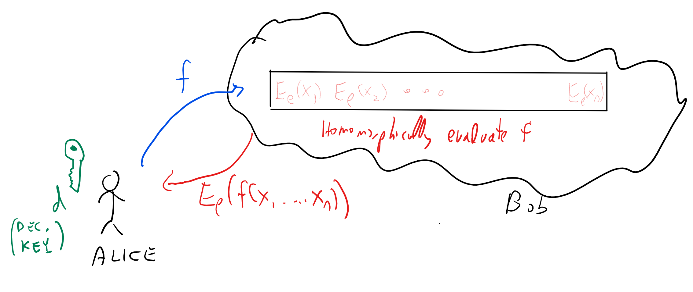
Already in 1978, Rivest, Adleman and Dertouzos considered this problem of a business that wishes to use a “commercial time-sharing service” to store some sensitive data. They envisioned a potential solution for this task which they called a privacy homomorphism. This notion later became known as fully homomorphic encryption (FHE) which is an encryption that allows a party (such as the cloud provider) that does not know the secret key to modify a ciphertext \(c\) encrypting \(x\) to a ciphertext \(c'\) encrypting \(f(x)\) for every efficiently computable \(f()\). In particular in our scenario above (see Figure 14.1), such a scheme will allow Bob, given an encryption of \(x\), to compute the encryption of \(f(x)\) and send this ciphertext to Alice without ever getting the secret key and so without ever learning anything about \(x\) (or \(f(x)\) for that matter).
Unlike the case of a trapdoor function, where it only took a year for Diffie and Hellman’s challenge to be answered by RSA, in the case of fully homomorphic encryption for more than 30 years cryptographers had no constructions achieving this goal. In fact, some people suspected that there is something inherently incompatible between the security of an encryption scheme and the ability of a user to perform all these operations on ciphertexts. Stanford cryptographer Dan Boneh used to joke to incoming graduate students that he will immediately sign the thesis of anyone who came up with a fully homomorphic encryption. But he never expected that he will actually encounter such a thesis, until in 2009, Boneh’s student Craig Gentry released a paper doing just that. Gentry’s paper shook the world of cryptography, and instigated a flurry of research results making his scheme more efficient, reducing the assumptions it relied on, extending and applying it, and much more. In particular, Brakerski and Vaikuntanathan managed to obtain a fully homomorphic encryption scheme based only on the Learning with Error (LWE) assumption we have seen before.
Although there is a number of implementations for (partially and) fully homomorphic encryption (see this list), there is still much work to be done in order to realize the full practical potential of FHE. For a comparable level of security, the encryption and decryption operations of a fully homomorphic encryption scheme are several orders of magnitude slower than a conventional public key system, and (depending on its complexity) homomorphically evaluating a circuit can be significantly more taxing. However, this is a fast evolving field, and already since 2009 significant optimizations have been discovered that reduced the computational and storage overhead by many orders of magnitudes. As in public key encryption, one would imagine that for larger data one would use a “hybrid” approach of combining FHE with symmetric encryption, though one might need to come up with tailor-made symmetric encryption schemes that can be efficiently evaluated.1 Homomorphically evaluations of approximate computation, which can be useful for machine learning, can be done more efficiently.
In this lecture and the next one we will focus on the fully homomorphic encryption schemes that are easiest to describe, rather than the ones that are most efficient (though the efficient schemes share many similarities with the ones we will talk about). As is generally the case for lattice based encryption, the current most efficient schemes are based on ideal lattices and on assumptions such as ring LWE or the security of the NTRU cryptosystem.2
To take the distance between theory and practice in perspective, it might be useful to consider the case of verifying computation. In the early 1990’s researchers (motivated initially by zero knowledge proofs) came up with the notion of probabilistically checkable proofs (PCP’s) which could yield in principle extremely succinct ways to check correctness of computation.
Probabilistically checkable proofs can be thought of as “souped up” versions of NP completeness reductions and like these reductions, have been mostly used for negative results, especially since the initial proofs were extremely complicated and also included enormous hidden constants. However, with time people have slowly understood these better and made them more efficient (e.g., see this survey) and it has now reached the point where these results, are practical (see also this) and in fact these ideas underlieat least two startups. Overall, constructions for verifying computation have improved by at least 20 orders of magnitude over the last two decades. (We will talk about some of these constructions later in this course.) If progress on fully homomorphic encryption follows a similar trajectory, then we can expect the road to practical utility to be very long, but there is hope that it’s not a “bridge to nowhere”.
Since large scale fully homomorphic encryption is still impractical, people have been trying to achieve at least weaker security goals using certain assumptions. In particular Intel chips have so called “Secure enclaves” which one can think of as a somewhat tamper-protected region of the processor that is supposed to be out of reach for the outside world. The idea is that a cloud provider client would treat this enclave as a trusted party that it can communicate with through the cloud provider. The client can store their data on the cloud encrypted with some key \(k\), and then set up a secure channel with the enclave using an authenticated key exchange protocol, and send \(k\) over. Then, when the client sends over a function \(f\) to the cloud provider, the latter party can simulate FHE by asking the enclave to compute the encryption of \(f(x)\) given the encryption of \(x\). In this solution ultimately the private key does reside on the cloud provider’s computers, and the client has to trust the security of the enclave. In practice, this could provide reasonable security against remote hackers, but (unlike FHE) probably not against sophisticated attackers (e.g., governments) that have physical access to the server.
Defining fully homomorphic encryption
We start by defining partially homomorphic encryption. We focus on encryption for single bits. This is without loss of generality for CPA security (CCA security is anyway ruled out for homomorphic encryption- can you see why?), though there are more efficient constructions that encrypt several bits at a time.
Let \(\mathcal{F} = \cup \mathcal{F}_\ell\) be a class of functions where every \(f\in\mathcal{F}_\ell\) maps \(\{0,1\}^\ell\) to \(\{0,1\}\).
An \(\mathcal{F}\)-homomorphic public key encryption scheme is a CPA secure public key encryption scheme \((G,E,D)\) such that there exists a polynomial-time algorithm \(\ensuremath{\mathit{EVAL}}:\{0,1\}^* \rightarrow \{0,1\}^*\) such that for every \((e,d)=G(1^n)\), \(\ell=poly(n)\), \(x_1,\ldots,x_\ell \in \{0,1\}\), and \(f\in \mathcal{F}_\ell\) of description size \(|f|\) at most \(poly(\ell)\) it holds that:
\(c=\ensuremath{\mathit{EVAL}}_e(f,E_e(x_1),\ldots,E_e(x_\ell))\) has length at most \(n\).
\(D_d(c)=f(x_1,\ldots,x_\ell)\).
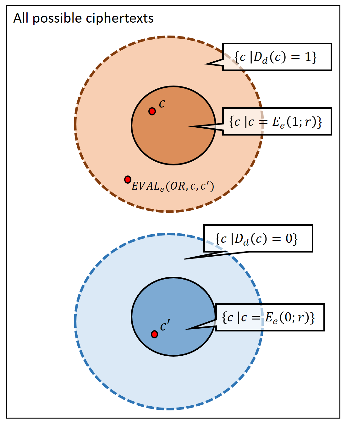
Please stop and verify you understand the definition. In particular you should understand why some bound on the length of the output of \(\ensuremath{\mathit{EVAL}}\) is needed to rule out trivial constructions that are the analogous of the cloud provider sending over to Alice the entire encrypted database every time she wants to evaluate a function of it. By artificially increasing the randomness for the key generation algorithm, this is equivalent to requiring that \(|c| \leq p(n)\) for some fixed polynomial \(p(\cdot)\) that does not grow with \(\ell\) or \(|f|\). You should also understand the distinction between ciphertexts that are the output of the encryption algorithm on the plaintext \(b\), and ciphertexts that decrypt to \(b\), see Figure 14.2.
A fully homomomorphic encryption is simply a partially homomorphic encryption scheme for the family \(\mathcal{F}\) of all functions, where the description of a function is as a circuit (say composed of NAND gates, which are known to be a universal basis).
Another application: fully homomorphic encryption for verifying computation
The canonical application of fully homomorphic encryption is for a client to store encrypted data \(E(x)\) on a server, send a function \(f\) to the server, and get back the encryption \(E(f(x))\) of \(f(x)\). This ensures that the server does not learn any information about \(x\), but does not ensure that it actually computes the correct function!
Here is a cute protocol to achieve the latter goal (due to Chung Kalai and Vadhan). Curiously the protocol involves “doubly encrypting” the input, and homomorphically evaluating the \(\ensuremath{\mathit{EVAL}}\) function itself.
Assumptions: We assume that all functions \(f\) that the client will be interested in can be described by a string of length \(n\).
Preprocessing: The client generates a pair of keys \((e,d)\). In the initial stage the client computes the encrypted database \(\overline{c}=E_e(x)\) and sends \(\overline{c},e\) to the server. It also computes \(c^* = E_e(f^*)\) for some function \(f^*\) as well as \(c^{**}=\ensuremath{\mathit{EVAL}}_{e}(eval,c^*\|\overline{c})\) for that \(f^*\) and keeps \(c^*,c^{**}\) for herself, where \(eval(f,x)=f(x)\) is the circuit evaluation function.
Client query: To ask for an evaluation of \(f\), the client generates a new random FHE keypair \((e',d')\), chooses \(b \leftarrow_R \{0,1\}\) and lets \(c_b = E_{e'}(E_e(f))\) and \(c_{1-b}=E_{e'}(c^*)\). It sends the triple \(e',c_0,c_1\) to the server.
Server response: Given the queries \(c_0,c_1\), the server defines the function \(g:\{0,1\}^* \rightarrow \{0,1\}^*\) where \(g(c)=\ensuremath{\mathit{EVAL}}_e(eval,c\|\overline{c})\) (for the fixed \(\overline{c}\) received) and computes \(c'_0,c'_1\) where \(c'_b = \ensuremath{\mathit{EVAL}}_{e'}(g,c_b)\). (Please pause here and make sure you understand what this step is doing! Note that we use here crucially the fact that \(\ensuremath{\mathit{EVAL}}\) itself is a polynomial time computation.)
Client check: Client checks whether \(D_{d'}(c'_{1-b})=c^{**}\) and if so accepts \(D_d(D_{d'}(c'_b))\) as the answer.
We claim that if the server cheats then the client will detect this with probability \(1/2 - negl(n)\). Working this out is a great exercise. The probability of detection can be amplified to \(1-negl(n)\) using appropriate repetition, see the paper for details.
Example: An XOR homomorphic encryption
It turns out that Regev’s LWE-based encryption LWEENC we saw before is homomorphic with respect to the class of linear (mod 2) functions. Let us recall the LWE assumption and the encryption scheme based on it.
Let \(q=q(n)\) be some function mapping the natural numbers to primes. The \(q(n)\)-decision learning with error (\(q(n)\)-dLWE) conjecture is the following: for every \(m=poly(n)\) there is a distribution \(\ensuremath{\mathit{LWE}}_q\) over pairs \((A,s)\) such that:
\(A\) is an \(m\times n\) matrix over \(\Z_q\) and \(s\in\Z_q^n\) satisfies \(s_1=\floor{\tfrac{q}{2}}\) and \(|(As)_i| \leq \sqrt{q}\) for every \(i\in \{1,\ldots, m\}\).
The distribution \(A\) where \((A,s)\) is sampled from \(\ensuremath{\mathit{LWE}}_q\) is computationally indistinguishable from the uniform distribution of \(m\times n\) matrices over \(\Z_q\).
The dLWE conjecture is that \(q(n)\)-dLWE holds for every \(q(n)\) that is at most \(poly(n)\). This is not exactly the same phrasing we used before, but as we sketch below, it is essentially equivalent to it. One can also make the stronger conjecture that \(q(n)\)-dLWE holds even for \(q(n)\) that is super polynomial in \(n\) (e.g., \(q(n)\) magnitude roughly \(2^n\) - note that such a number can still be described in \(n\) bits and we can still efficiently perform operations such as addition and multiplication modulo \(q\)). This stronger conjecture also seems well supported by evidence and we will use it in future lectures.
It is a good idea for you to pause here and try to show the equivalence on your own.
Equivalence between LWE and DLWE: The reason the two conjectures are equivalent are the following. Before we phrased the conjecture as recovering \(s\) from a pair \((A',y)\) where \(y=A's'+e\) and \(|e_i|\leq \delta q\) for every \(i\). We then showed a search to decision reduction (Theorem 11.2) demonstrating that this is equivalent to the task of distinguishing between this case and the case that \(y\) is a random vector. If we now let \(\alpha = \floor{\tfrac{q}{2}}\) and \(\beta = \alpha^{-1} \pmod q\), and consider the matrix \(A=(-\beta y|A')\) and the column vector \(s=\binom{\alpha}{s'}\) we see that \(As = e\). Note that if \(y\) is a random vector in \(\Z_q^m\) then so is \(-\beta y\) and so the current form of the conjecture follows from the previous one. (To reduce the number of free parameters, we fixed \(\delta\) to equal \(1/\sqrt{q}\); in this form the conjecture becomes stronger as \(q\) grows.)
A linearly-homomorphic encryption scheme: The following variant of the LWE-ENC described in Section 11.4 turns out to be linearly homomorphic:
LWE-ENC’ encryption:
Key generation: Choose \((A,s)\) from \(\ensuremath{\mathit{LWE}}_q\) where \(m\) satisfies \(q^{1/4} \gg m \log q \gg n\).
To encrypt \(b\in\{0,1\}\), choose \(w\in\{0,1\}^m\) and output \(w^\top A + (b,0,\ldots,0)\).
To decrypt \(c\in\Z_q^n\), output \(0\) iff \(|\langle c,s \rangle| \leq q/10\), where for \(x\in\Z_q\) we defined \(|x| = \min \{ x , q-x \}\). (Recall that the first coordinate of \(s\) is \(\floor{q/2}\).)
The decryption algorithm recovers the original plaintext since \(\langle c,s \rangle= w^\top A s + s_1 b\) and \(|w^\top A s| \leq m\sqrt{q} \ll q\). It turns out that this scheme is homomorphic with respect to the class of linear functions modulo \(2\). Specifically we make the following claim:
For every \(\ell \ll q^{1/4}\), there is an algorithm \(\ensuremath{\mathit{EVAL}}_\ell\) that on input \(c_1,\ldots,c_\ell\) which are LWEENC-encryptions of the bits \(b_1,\ldots,b_\ell \in \{0,1\}\), outputs a ciphertext \(c\) whose decryption is \(b_1 \oplus \cdots \oplus b_\ell\).
This claim is not hard to prove, but working it out for yourself can be a good way to get more familiarity with LWE-ENC’ and the kind of manipulations we’ll be making time and again in the constructions of many lattice based cryptographic primitives. Recall that a ciphertext \(c\) of LWE-ENC’ is a vector in \(\Z_q^n\). Try to show that \(c = c_1 + \cdots +c_\ell\) (where addition is done as vectors in \(\Z_q\)) will be the encryption of \(b_1 \oplus \cdots \oplus b_\ell\). Note that if \(q\) is super polynomial in \(n\) then \(\ell\) can be an arbitrarily large polynomial in \(n\).
The proof is quite simple. \(\ensuremath{\mathit{EVAL}}\) will simply add the ciphertexts as vectors in \(\Z_q\). If \(c = \sum c_i\) then
Since \(|\floor{\tfrac{q}{2}}- \tfrac{q}{2}|<1\), adding at most \(\ell\) terms of this difference adds at most \(\ell\), and so we can also write
If \(\sum b_i\) is even then \(\sum b_i \tfrac{q}{2}\) is an integer multiple of \(q\) and hence in this case \(|\langle c,s \rangle| \ll q\). If \(\sum b_i\) is odd \(\floor{\sum b_i \tfrac{q}{2}} = \floor{q/2} \mod q\) and so in this case \(|\langle c,s \rangle| = q/2 \pm o(q) > q/10\).
Several other encryption schemes are also homomorphic with respect to linear functions. Even before Gentry’s construction there were constructions of encryption schemes that are homomorphic with respect to somewhat larger classes (e.g., quadratic functions by Boneh, Goh and Nissim) but not significantly so.
Abstraction: A trapdoor pseudorandom generator.
It is instructive to consider the following abstraction (which we’ll use in the next lecture) of the above encryption scheme as a trapdoor generator (see Figure 14.3). On input \(1^n\) the key generation algorithm outputs a vector \(s\in\Z_q^m\) with \(s_1 = \floor{\tfrac{q}{2}}\) and a probabilistic algorithm \(G_s\) such that the following holds:
Any polynomial number of samples from the distribution \(G_s(1^n)\) is computationally indistinguishable from independent samples from the uniform distribution over \(\Z_q^n\).
If \(c\) is output by \(G_s(1^n)\) then \(|\langle c,s \rangle| \leq n\sqrt{q}\).
The generator \(G_s\) picks \(w \leftarrow_R \{0,1\}^m\) to \(w^\top A\). Its output will look pseudorandom but will satisfy the condition \(|\langle G_s(1^n),s \rangle| \leq n\sqrt{q}\) with probability \(1\) over the choice of \(w\). Thus \(s\) can be thought of a “trapdoor” for the generator that allows us to distinguish between a random vector \(c\in \Z_q^n\) (that with high probability would satisfy \(|\langle c,s \rangle| \gg n\sqrt{q}\), assuming \(q \gg n^2\)) and an output of the generator.
We use \(G_s\) to encrypt a bit \(b\) by letting \(c \leftarrow_R G_s(1^n)\) and outputting \(c + (b,0,\ldots,0)^\top\). While our particular implementation mapped \(G_s(w)= w^\top A\), we can ignore these implementation details in the forgoing.
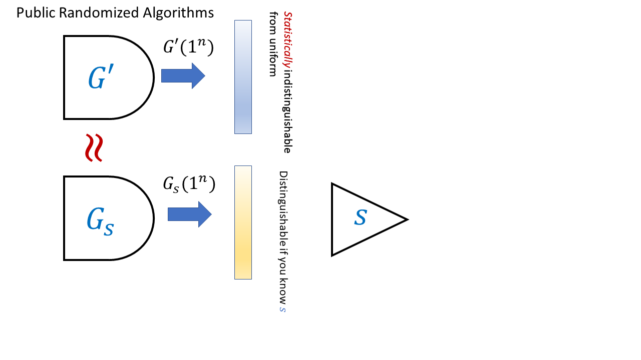
Our LWE-based trapdoor generator satisfies the following stronger property: we can generate an alternative generator \(G'\) such that the description of \(G'\) is indistinguishable from the description of \(G_s\) but such that \(G'\) actually does produce (up to exponentially small statistical error) the uniform distribution over \(\Z_q^n\). We can do so by sampling \(A\) completely at random instead of from the \(\ensuremath{\mathit{LWE}}_q\) distribution. We can define trapdoor generators formally as follows
A trapdoor generator is a pair of randomized algorithms \(\ensuremath{\mathit{GEN}},\ensuremath{\mathit{GEN}}'\) that satisfy the following:
On input \(1^n\), \(\ensuremath{\mathit{GEN}}\) outputs a pair \((G_s,s)\) where \(G_s\) is a string describing a randomized circuit. The circuit \(G_s\) takes \(1^n\) as input and outputs a (randomly chosen) string of length \(t\) where \(t=t(n)\) is some polynomial.
On input \(1^n\), \(\ensuremath{\mathit{GEN}}'\) outputs \(G'\) where \(G'\) is a string describing a randomized circuit with the same inputs and outputs.
The distributions \(\ensuremath{\mathit{GEN}}(1^n)_1\) (i.e., the first output of \(\ensuremath{\mathit{GEN}}(1^n)\)) and \(\ensuremath{\mathit{GEN}}'(1^n)_1\) are computationally indistinguishable. (These are both distributions over circuits.)
With probability \(1-negl(n)\) over the choice of \(G'\) output by \(\ensuremath{\mathit{GEN}}'\), the distribution \(G'(1^n)\) is statistically indistinguishable (i.e., within \(negl(n)\) total variation distance) from \(U_t\) (i.e., the uniform distribution over \(\{0,1\}^t\)).
There is an efficient algorithm \(T\) such that for every pair \((G_s,s)\) output by \(\ensuremath{\mathit{GEN}}\), \(\Pr[ T(s,G_s(1^n))=1] \geq 1- negl(n)\) (where this probability is over the internal randomness used by \(G_s\) on the input \(1^n\)) but \(\Pr[ T(s,U_t)=1] \leq 1/3\).3
This is not an easy definition to parse, but looking at Figure 14.3 can help. Make sure you understand why \(\ensuremath{\mathit{LWEENC}}\) gives rise to a trapdoor generator satisfying all the conditions of Definition 14.6.
In the above we use the notion of a “trapdoor” in the pseudorandom generator as a mathematical abstraction, but generators with actual trapdoors have arisen in practice. In 2007 the National Institute of Standards (NIST) released standards for pseudorandom generators. Pseudorandom generators are the quintessential private key primitive, typically built out of hash functions, block ciphers, and such and so it was surprising that NIST included in the list a pseudorandom generator based on public key tools - the Dual EC DRBG generator based on elliptic curve cryptography. This was already strange but became even more worrying when Microsoft researchers Dan Shumow and Niels Ferguson showed that this generator could have a trapdoor in the sense that it contained some hardwired constants that if generated in a particular way, there would be some information that (just like in \(G_s\) above) allows to distinguish the generator from random (see here for a 2007 blog post on this issue). We learned more about this when leaks from the Snowden document showed that the NSA secretly paid 10 million dollars to RSA to make this generator the default option in their Bsafe software.
You’d think that this generator is long dead but it turns out to be the “gift that keeps on giving”. In December of 2015, Juniper systems announced that they have discovered a malicious code in their system, dating back to at least 2012 (possibly 2008), that would allow an attacker to surreptitiously decrypt all VPN traffic through their firewalls. The issue is that Juniper has been using the Dual EC DRBG and someone has managed to replace the constant they were using with another one, one that they presumably knew the trapdoor for (see here and here for more; of course unless you know to check for this, it’s very hard by looking at the code to see that one arbitrary looking constant has been replaced by another). Apparently, even though this is very surprising to many people in law enforcement and government, inserting back doors into cryptographic primitives might end up making them less secure. Some more details have emereged in this case in 2021, see this story and this Tweet thread.
From linear homomorphism to full homomorphism
Gentry’s breakthrough had two components:
First, he gave a scheme that is homomorphic with respect to arithmetic circuits (involving not just addition but also multiplications) of logarithmic depth.
Second, he showed the amazing “bootstrapping theorem” that if a scheme is homomorphic enough to evaluate its own decryption circuit, then it can be turned into a fully homomorphic encryption that can evaluate any function.
Combining these two insights led to his fully homomorphic encryption.4
In this lecture we will focus on the second component - the bootstrapping theorem. We will show a “partially homomorphic encryption” (based on a later work of Gentry, Sahai and Waters) that can fit that theorem in the next lecture.
Bootstrapping: Fully Homomorphic “escape velocity”
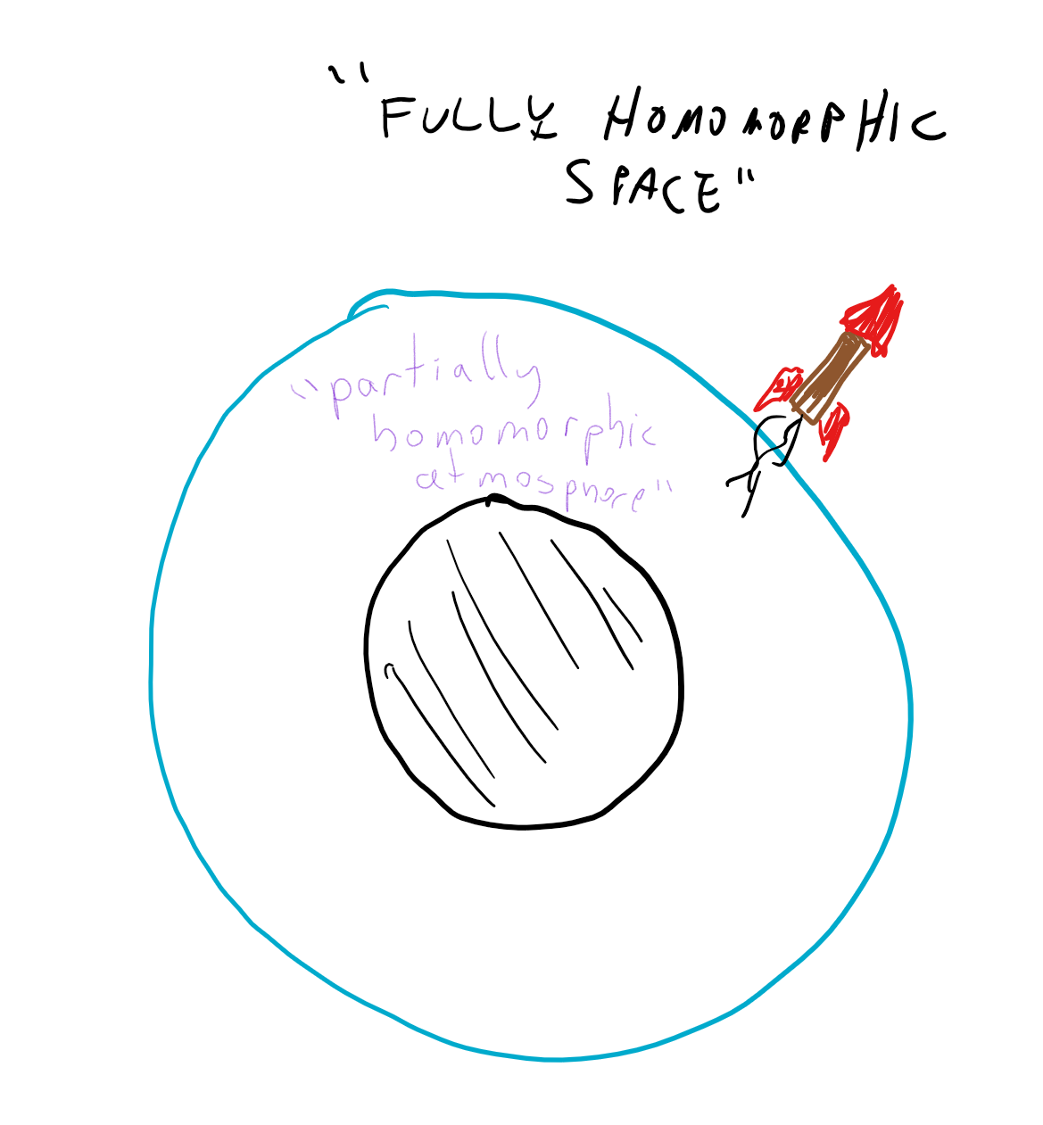
The bootstrapping theorem is quite surprising. A priori you might expect that given that a homomorphic encryption for linear functions was not trivial to do, a homomorphic encryption for quadratics would be harder, cubics even harder and so on and so forth. But it turns out that there is some special degree \(t^*\) such that if we obtain homomorphic encryption for degree \(t^*\) polynomials then we can obtain fully homomorphic encryption that works for all functions. (Specifically, if the decryption algorithm \(c \mapsto D_d(c)\) is a degree \(t\) polynomial, then homomorphically evaluating polynomials of degree \(t^*=2t\) will be sufficient.) That is, it turns out that once an encryption scheme is strong enough to homomorphically evaluate its own decryption algorithm then we can use it to obtain a fully homomorphic encryption by “pulling itself up by its own bootstraps”. One analogy is that at this point the encryption reaches “escape velocity” and we can continue onwards evaluating gates in perpetuity.
We now show the bootstrapping theorem:
Suppose that \((G,E,D)\) is a CPA circular5 secure partially homomorphic encryption scheme for the family \(\mathcal{F}\) and suppose that for every pair of ciphertexts \(c,c'\) the map \(d \mapsto D_d(c) \;\ensuremath{\mathit{NAND}}\; D_d(c')\) is in \(\mathcal{F}\). Then \((G,E,D)\) can be turned a fully homomorphic encryption scheme.
Radioactive legos analogy
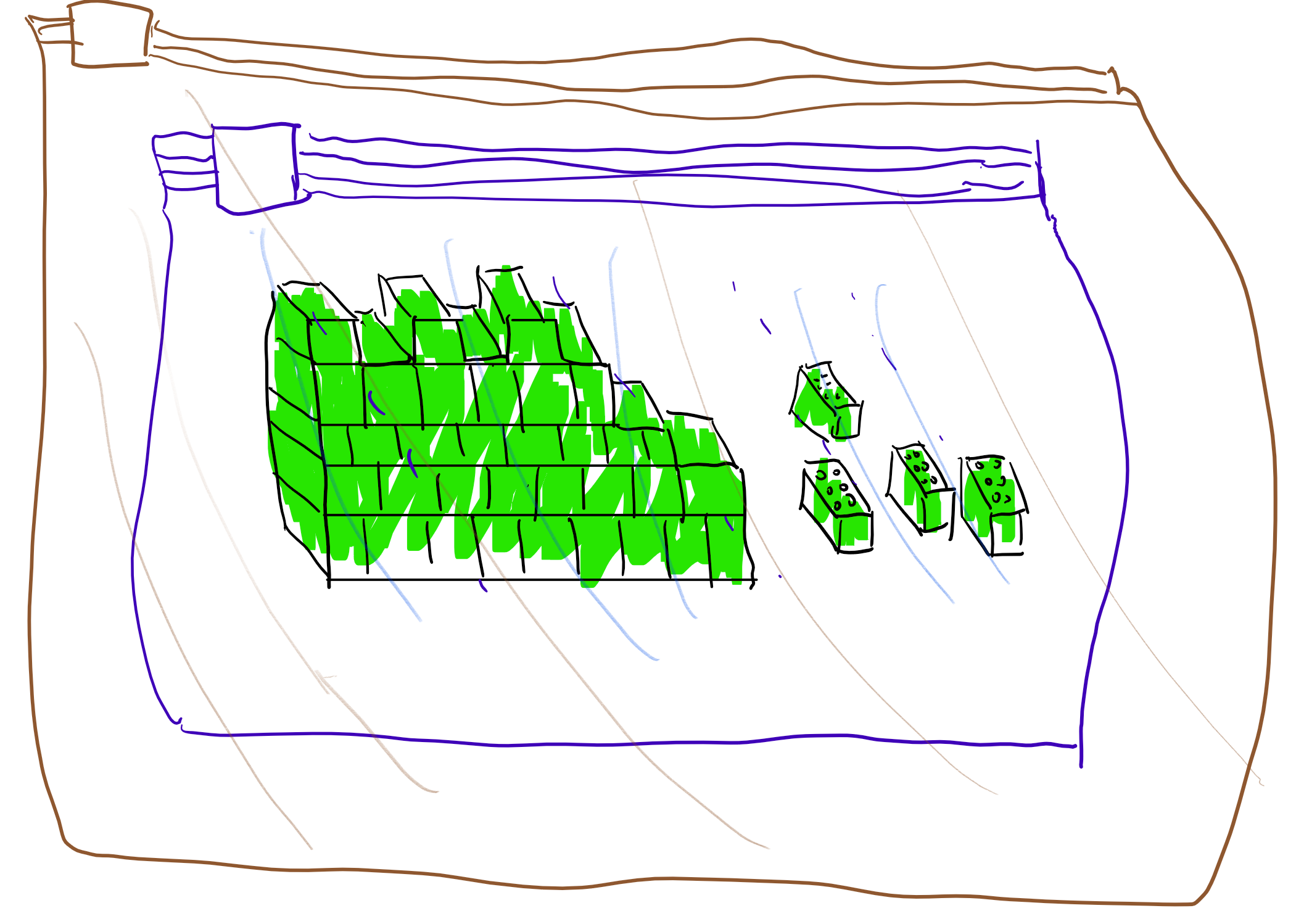
Here is one analogy for bootstrapping, inspired by Gentry’s survey. Suppose that you need to construct some complicated object from a highly toxic material (see Figure 14.5). For example you want to build a castle out of radio-active legos.
You are given a supply of sealed bags that are flexible enough so you can manipulate the object from outside the bag. However, each bag can only hold for \(10\) seconds of such manipulations before it leaks. The idea is that if you can open one bag inside another within \(9\) seconds then you can use the extra second to perform one step. By repeating this, you perform the manipulations for arbitrary length.
Specifically, suppose that you have completed \(i\) steps out of the total of \(T\), and now have the partially constructed castle inside a sealed bag \(B_i\). You now put the bag \(B_i\) inside a fresh bag \(B_{i+1}\). You now spend \(9\) seconds on opening the bag \(B_i\) inside the bag \(B_{i+1}\), and an extra second on performing the \(i+1\) step in the construction. At this point we have completed \(i+1\) steps and have the object in the bag \(B_{i+1}\), we can now continue by putting in the bag \(B_{i+2}\) and so on and so forth.
Proving the bootstrapping theorem
We now turn to the formal proof of Theorem 14.8
The idea behind the proof is simple but ingenious. Recall that the NAND gate \(b,b' \mapsto \neg(b \wedge b')\) is a universal gate that allows us to compute any function \(f:\{0,1\}^n\rightarrow\{0,1\}\) that can be efficiently computed. Thus, to obtain a fully homomorphic encryption it suffices to obtain a function \(\ensuremath{\mathit{NANDEVAL}}\) such that \(D_d(\ensuremath{\mathit{NANDEVAL}}(c,c'))=D_d(c) \;\ensuremath{\mathit{NAND}}\; D_d(c')\). (Note that this is stronger than the typical notion of homomorphic evaluation since we require that \(\ensuremath{\mathit{NANDEVAL}}\) outputs an encryption of \(b \;\ensuremath{\mathit{NAND}}\; b'\) when given any pair of ciphertexts that decrypt to \(b\) and \(b'\) respectively, regardless whether these ciphertexts were produced by the encryption algorithm or by some other method, including the \(\ensuremath{\mathit{NANDEVAL}}\) procedure itself.)
Thus to prove the theorem, we need to modify \((G,E,D)\) into an encryption scheme supporting the \(\ensuremath{\mathit{NANDEVAL}}\) operation. Our new scheme will use the same encryption algorithms \(E\) and \(D\) but the following modification \(G'\) of the key generation algorithm: after running \((d,e)=G(1^n)\), we will append to the public key an encryption \(c^* = E_e(d)\) of the secret key. We have now defined the key generation, encryption and decryption. CPA security follows from the security of the original scheme, where by circular security we refer exactly to the condition that the scheme is secure even if the adversary gets a single encryption of the public key.6 This latter condition is not known to be implied by standard CPA security but as far as we know is satisfied by all natural public key encryptions, including the LWE-based ones we will plug into this theorem later on.
So, now all that is left is to define the \(\ensuremath{\mathit{NANDEVAL}}\) operation. On input two ciphertexts \(c\) and \(c'\), we will construct the function \(f_{c,c'}:\{0,1\}^n\rightarrow\{0,1\}\) (where \(n\) is the length of the secret key) such that \(f_{c,c'}(d)=D_d(c) \;\ensuremath{\mathit{NAND}}\; D_d(c')\). It would be useful to pause at this point and make sure you understand what are the inputs to \(f_{c,c'}\), what are “hardwired constants” and what is its output. The ciphertexts \(c\) and \(c'\) are simply treated as fixed strings and are not part of the input to \(f_{c,c'}\). Rather \(f_{c,c'}\) is a function (depending on the strings \(c,c'\)) that maps the secret key into a bit. When running \(\ensuremath{\mathit{NANDEVAL}}\) we of course do not know the secret key \(d\), but we can still design a circuit that computes this function \(f_{c,c'}\). Now \(\ensuremath{\mathit{NANDEVAL}}(c,c')\) will simply be defined as \(\ensuremath{\mathit{EVAL}}(f_{c,c'},c^*)\). Since \(c^* = E_e(d)\), we get that
Don’t let the short proof fool you. This theorem is quite deep and subtle, and requires some reading and re-reading to truly “get” it.
- ↩
In 2015 the state of art on homomorphically evaluating AES was about 6 seconds of computation per block using about 4GB memory total for 180 blocks. See also this paper. In contrast, modern processors can evaluate 10s-100s millions of AES blocks per second.
- ↩
As we mentioned before, as a general rule of thumb, the difference between the ideal schemes and the one that we describe is that in the ideal setting one deals with structured matrices that have a compact representation as a single vector and also enable fast FFT-like matrix-vector multiplication. This saves a factor of about \(n\) in the storage and computation requirements (where \(n\) is the dimension of the subspace/lattice). However, there can be some subtle security implications for ideal lattices as well, see e.g., here, here, here, and here.
- ↩
The choice of \(1/3\) is arbitrary, and can be amplified as needed.
- ↩
The story is a bit more complex than that. Frustratingly, the decryption circuit of Gentry’s basic scheme was just a little bit too deep for the bootstrapping theorem to apply. A lesser man, such as yours truly, would at this point surmise that fully homomprphic encryption was just not meant to be, and perhaps take up knitting or playing bridge as an alternative hobby. However, Craig persevered and managed to come up with a way to “squash” the decryption circuit so it can fit the bootstrapping parameters. Follow up works, and in particular the paper of Brakerski and Vaikuntanathan, managed to get schemes with much better relation between the homomorphism depth and decryption circuit, and hence avoid the need for squashing and also improve the security assumptions.
- ↩
You can ignore the condition of circular security in a first read - we will discuss it later.
- ↩
Without this assumption we can still obtain a form of FHE known as a leveled FHE where the size of the public key grows with the depth of the circuit to be evaluated. We can do this by having \(\ell\) public keys where \(\ell\) is the depth we want to evaluate, and encrypt the private key of the \(i^{th}\) key with the \(i+1^{st}\) public key. However, since circular security seems quite likely to hold, we ignore this extra complication in the rest of the discussion.
Comments
Comments are posted on the GitHub repository using the utteranc.es app. A GitHub login is required to comment. If you don't want to authorize the app to post on your behalf, you can also comment directly on the GitHub issue for this page.
Compiled on 11/17/2021 22:36:02
Copyright 2021, Boaz Barak.

This work is
licensed under a Creative Commons
Attribution-NonCommercial-NoDerivatives 4.0 International License.
Produced using pandoc and panflute with templates derived from gitbook and bookdown.